Table of Contents
Open Table of Contents
Introduction
In this blog post, we will cover the basics of statistics and how to apply them in Python through a practical lens. Specifically, we’ll work through a series of practice problems based on a realistic scenario involving machine learning experiments. We’ll use Python and various statistical techniques to analyze the results and draw meaningful conclusions.
Scenario: Comparing a Novel Machine Learning Method to a Baseline
Imagine you’re a research scientist at a leading AI company, and you’ve developed a new machine learning method that you believe outperforms the current baseline model. To test your hypothesis, you’ve run a series of experiments comparing your novel method to the baseline across different datasets and metrics.
Our task is to analyze the results of these experiments using various statistical techniques and draw conclusions about the performance of your novel method compared to the baseline.
Experiment Results
You have the following data from your experiments, comparing the accuracy of your novel method to the baseline across 10 different datasets:
Mock Experiment Data Generation
def generate_realistic_ml_data(n_experiments=50, random_seed=42, with_issues=True):
    """
    Generate synthetic ML experiment data in long format, with multiple methods
    and experimental runs.
    """
    np.random.seed(random_seed)

    # Define methods and their characteristics
    methods = {
        "Baseline": {"param_efficiency": 1.0, "variance": 0.02},
        "Novel_A": {  # Our primary novel method
            "param_efficiency": 1.15,  # 15% more parameter efficient
            "variance": 0.02,
        },
        "Novel_B": {  # An alternative approach
            "param_efficiency": 1.10,  # 10% more parameter efficient
            "variance": 0.015,
        },
        "CompetitorX": {  # Published SOTA method
            "param_efficiency": 1.12,
            "variance": 0.02,
        },
    }

    # Generate base experiments
    experiments = []

    for exp_id in range(n_experiments):
        # Base parameters for this experiment
        log_params = np.random.uniform(
            low=np.log10(1e7),  # 10M parameters
            high=np.log10(1e10),  # 10B parameters
        )
        base_params = 10**log_params

        log_tokens = np.random.uniform(
            low=np.log10(1e9),  # 1B tokens
            high=np.log10(1e12),  # 1T tokens
        )
        base_tokens = 10**log_tokens

        dataset_type = np.random.choice(
            ["tabular", "image", "text", "time-series"], p=[0.2, 0.3, 0.4, 0.1]
        )

        # Calculate base theoretical accuracy
        base_loss = 2.0
        param_factor = 0.1 * np.log10(base_params / 1e7)
        token_factor = 0.1 * np.log10(base_tokens / 1e9)
        theoretical_accuracy = 0.85 - (base_loss - param_factor - token_factor) * 0.1

        # Generate results for each method
        for method_name, method_props in methods.items():
            # Some methods might fail occasionally
            if np.random.random() < 0.05:  # 5% failure rate
                continue

            # Add method-specific variation
            method_accuracy = theoretical_accuracy * method_props[
                "param_efficiency"
            ] + np.random.normal(0, method_props["variance"])
            method_accuracy = np.clip(method_accuracy, 0, 1)

            # Vary parameters and tokens slightly between methods
            method_params = base_params * np.random.uniform(0.95, 1.05)
            method_tokens = base_tokens * np.random.uniform(0.95, 1.05)

            experiment = {
                "Experiment_ID": exp_id + 1,
                "Method": method_name,
                "Dataset_Type": dataset_type,
                "Model_Parameters": int(method_params),
                "Training_Tokens": int(method_tokens),
                "Accuracy": method_accuracy,
                "GPU_Memory_GB": np.clip(method_params / 1e8, 8, 80)
                + np.random.normal(0, 2),
                "Compute_Cost_USD": (method_params * method_tokens) / 1e12 * 0.1
                + np.random.lognormal(0, 0.5),
            }
            experiments.append(experiment)

    df_raw = pd.DataFrame(experiments)

    if with_issues:
        # Add some realistic issues
        missing_indices = np.random.choice(len(df_raw), 10, replace=False)
        df_raw.loc[missing_indices, "Training_Tokens"] = np.nan  # type: ignore

        # Add some corrupted values
        corrupted_indices = np.random.choice(len(df_raw), 5, replace=False)
        df_raw.loc[corrupted_indices, "GPU_Memory_GB"] *= -1  # type: ignore

    return df_raw
df = generate_realistic_ml_data(n_experiments=50, random_seed=42, with_issues=True)
df.head()
>>>
   Experiment_ID       Method Dataset_Type  Model_Parameters  Training_Tokens  Accuracy  GPU_Memory_GB  Compute_Cost_USD
0              1     Baseline         text         127054830     7.374991e+11  0.685075       7.531726      9.370285e+06
1              1      Novel_B         text         137348322     6.909820e+11  0.770245       7.073165      9.490523e+06
2              1  CompetitorX         text         130154015     7.194053e+11  0.720278       9.900739      9.363350e+06
3              2     Baseline         text         125806559     2.356161e+10  0.659825       8.244438      2.964213e+05
4              2      Novel_A         text         127942212     2.320614e+10  0.763861       7.416613      2.969055e+05
Data Quality Checks
Before diving into analysis, let’s perform some basic data quality checks:
import numpy as np
import pandas as pd


def check_data_quality(df: pd.DataFrame):
    print("1. Basic Information:")
    print("-" * 80)
    print(df.info())

    print("2. Missing or NaN Values:")
    print("-" * 80)
    print(df.isnull().sum())

    print("3. Basic Statistics:")
    print("-" * 80)
    print(df.describe())

    print("4. Value Ranges Check:")
    print("-" * 80)
    numeric_cols = df.select_dtypes(include=[np.number]).columns
print(df[numeric_cols].describe().loc[["min", "max"]].transpose())RangeIndex: 185 entries, 0 to 184
Data columns (total 9 columns):
# Column Non-Null Count Dtype
--- ------ -------------- -----
0 Unnamed: 0 185 non-null int64
1 Experiment_ID 185 non-null int64
2 Method 185 non-null object
3 Dataset_Type 185 non-null object
4 Model_Parameters 185 non-null int64
5 Training_Tokens 175 non-null float64
6 Accuracy 185 non-null float64
7 GPU_Memory_GB 185 non-null float64
8 Compute_Cost_USD 185 non-null float64
dtypes: float64(4), int64(3), object(2)
memory usage: 13.1+ KB
None2. Missing or NaN Values:
--------------------------------------------------------------------------------
Unnamed: 0 0
Experiment_ID 0
Method 0
Dataset_Type 0
Model_Parameters 0
Training_Tokens 10
Accuracy 0
GPU_Memory_GB 0
Compute_Cost_USD 0
dtype: int643. Basic Statistics:
--------------------------------------------------------------------------------
Unnamed: 0 Experiment_ID Model_Parameters Training_Tokens \
count 185.000000 185.000000 1.850000e+02 1.750000e+02
mean 92.000000 25.632432 1.388827e+09 1.831435e+11
std 53.549043 14.275817 2.217385e+09 2.535071e+11
min 0.000000 1.000000 1.197368e+07 1.097568e+09
25% 46.000000 13.000000 6.421651e+07 5.069342e+09
50% 92.000000 26.000000 3.348831e+08 5.108024e+10
75% 138.000000 38.000000 1.259502e+09 2.411515e+11
max 184.000000 50.000000 9.501760e+09 8.846393e+11
Accuracy GPU_Memory_GB Compute_Cost_USD
count 185.000000 185.000000 1.850000e+02
mean 0.745665 16.486504 2.063836e+07
std 0.044442 20.304146 5.771334e+07
min 0.644119 -69.491861 5.449061e+03
25% 0.720278 7.380907 2.991098e+05
50% 0.751186 9.543397 9.762707e+05
75% 0.777487 14.014378 9.363350e+06
max 0.845723 80.540914 2.827613e+084. Value Ranges Check:
--------------------------------------------------------------------------------
min max
Unnamed: 0 0.000000e+00 1.840000e+02
Experiment_ID 1.000000e+00 5.000000e+01
Model_Parameters 1.197368e+07 9.501760e+09
Training_Tokens 1.097568e+09 8.846393e+11
Accuracy 6.441188e-01 8.457234e-01
GPU_Memory_GB -6.949186e+01 8.054091e+01
Compute_Cost_USD 5.449061e+03 2.827613e+08Data Cleaning and Preprocessing
Let’s handle the common data issues we identified:
def clean_dataset(df):
    df_clean = df.copy()

    # 1. Handle missing values
    # Fill missing values with median
    median_tokens = df["Training_Tokens"].median()
    df["Training_Tokens"] = df["Training_Tokens"].fillna(median_tokens)


    # 2. Fix impossible values
    df_clean.loc[df_clean['Baseline_Accuracy'] > 1, 'Baseline_Accuracy'] = 1.0
    df_clean.loc[df_clean['Novel_Method_Accuracy'] > 1, 'Novel_Method_Accuracy'] = 1.0

    # 3. Handle outliers using IQR method
    def remove_outliers(series):
        Q1 = series.quantile(0.25)
        Q3 = series.quantile(0.75)
        IQR = Q3 - Q1
        lower_bound = Q1 - 1.5 * IQR
        upper_bound = Q3 + 1.5 * IQR
        return np.where(series.between(lower_bound, upper_bound), series, series.median())

    numerical_cols = ['GPU_Memory_GB', 'Training_Time_Hours']
    for col in numerical_cols:
        df_clean[col] = remove_outliers(df_clean[col])

    return df_clean

df = clean_dataset(df_raw)Descriptive Statistics and Data Visualization
First, let’s compute some basic statistical measures and plot some data visualizations using Pandas and Matplotlib.
Mean, Median, Mode
Let’s start with some definitions and calculations for our dataset.
Definitions
-
Mean ():
- The average value of a dataset, calculated by summing all values and dividing by the number of data points.
- The first moment of a probability distribution, equivalent to the expected value for discrete distributions or for continuous distributions. For a finite dataset,
-
Median: The middle value when a dataset is ordered from least to greatest.
-
Mode: The most frequently occurring value in a dataset.
-
Standard Deviation .
- A measure of the amount of variation or dispersion of a set of values.
- The square root of the variance (second central moment).
- Equivalent to .
-
Variance: (for a finite dataset)
- The average of the squared differences from the mean.
- The second central moment of a probability distribution
- Defined as , measuring the expected squared deviation from the mean.
Now, let’s calculate these statistics for our experimental results:
# Group by method
methods = {name: data for name, data in df.groupby("Method")}

for name, method in methods.items():
    print(name)
    print(method.describe())
Sample vs. Population Statistics: Understanding the Difference
When working with data, we often need to distinguish between population parameters and sample statistics. This distinction is crucial because we rarely have access to an entire population and must make inferences from samples.
The uncorrected sample variance and standard deviation are biased estimators of the population variance and standard deviation that tend to underestimate the true value. To correct for this bias, we divide by instead of in the sample variance formula. This correction factor is known as Bessel’s correction or the “degrees of freedom” adjustment.
Sample variance (corrected):
Sample standard deviation (corrected):
Note:
- Samples tend to be closer to their sample mean than to the population mean
- Using instead of makes the sample variance an unbiased estimator of the population variance
- This correction becomes less important as the sample size increases
In python, you can calculate the corrected sample standard deviation using the ddof parameter in np.std():
import numpy as np

# Population statistics
population_mean = np.mean(data)
population_var = np.var(data, ddof=0)    # ddof=0 for population
population_std = np.std(data, ddof=0)

# Sample statistics
sample_mean = np.mean(data)
sample_var = np.var(data, ddof=1)        # ddof=1 for sample
sample_std = np.std(data, ddof=1)
Standard Error of the Mean (SEM)
The standard error of the mean (SEM) tells us how precise our sample mean is as an estimate of the population mean. It’s calculated as:
where
- is the sample standard deviation
- is the sample size.
This relationship shows us something crucial: our uncertainty about the true population mean decreases with: (1) larger sample sizes ( term) and (2) less variable data ( term).
Thus, a smaller SEM indicates that the sample mean is a more precise estimate of the true population mean.
In Python, you can calculate the SEM using the formula above:
import numpy as np

# Calculate the standard error of the mean (SEM)
sample_std = np.std(data, ddof=1)  # ddof=1 for sample standard deviation
sem = sample_std / np.sqrt(len(data))
The SEM is crucial for constructing confidence intervals and performing hypothesis tests. A smaller SEM indicates that the sample mean is a more precise estimate of the true population mean.
When we’re dealing with small sample sizes , we often use the t-distribution instead of the normal distribution for inference. This is because the t-distribution accounts for the additional uncertainty when estimating the population standard deviation from a small sample.
Error Bars in Visualization
Error bars can represent different measures of uncertainty:
- Standard Deviation (shows spread of the data)
- Standard Error (shows uncertainty in the mean)
- Confidence Intervals (shows range of plausible population values) (we’ll cover this in the next section)
The choice depends on your message:
- Use SD to show data variability
- Use SEM to show precision of your mean estimate
- Use CI to show range of plausible population values
Visualizing the Data
Now that we have our basic statistics, let’s create some visualizations to better understand our data.
methods = {name: data for name, data in df.groupby("Method")}

# Matplotlib boxplot

plt.figure(figsize=(10, 6))
plt.boxplot(
[data["Accuracy"] for data in methods.values()], tick_labels=list(methods.keys())
)
plt.ylabel("Accuracy")
plt.xlabel("Method")
plt.title("Model Accuracy by Method")
plt.show()
methods = {name: data for name, data in df.groupby("Method")}
# Seaborn boxplot
sns.boxplot(x="Method", y="Accuracy", data=df)
plt.title("Model Accuracy by Method")
plt.show()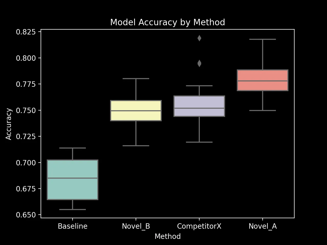
Boxplot of Model Accuracy by Method (seaborn output)
The boxplot above shows the distribution of model accuracy for each method. It provides a visual summary of the central tendency, spread, and skewness of the data. The line inside the box represents the median, while the box itself spans the interquartile range (IQR). The whiskers extend to the most extreme data points within 1.5 times the IQR from the box. Points outside this range are considered outliers. The plot strongly suggests that there are statistically significant differences between the methods.
In our next section on Hypothesis Testing, we’ll use these concepts to determine if the difference between our novel method and the baseline is statistically significant.
Hypothesis Testing
Next, let’s focus on formulating hypotheses and performing a paired t-test to compare the performance of two methods.
Formulating the Hypotheses
In our scenario, we want to test if our novel method significantly outperforms the baseline. We can formulate our hypotheses as follows:
-
Null Hypothesis (): There is no significant difference between the mean accuracy of the novel method and the baseline method. Mathematically: , where is the mean of the differences (Novel - Baseline).
-
Alternative Hypothesis (): The novel method has a significantly higher mean accuracy than the baseline method. Mathematically:
Student’s t-test
Student’s t-test is a statistical test used to test whether the difference between the response of two groups is statistically significant or not
Assumptions:
- The data is normally distributed
- The variances of the two groups are equal
- Independent observations (except for paired test)
t-statistic: The t-statistic measures the difference between the means of two paired samples relative to the variability within the samples. In other words, it is the ratio of the difference between the means to the standard error of that difference.
The formula for the t-statistic is given by:
It is very similar to the z-score but with the difference that t-statistic is used when the sample size is small or the population standard deviation is unknown (a t-test will converge to a Z-test as the dataset size increases).
Quick Decision Tree
Is your data paired/matched?
└─ Yes → Use Paired t-test
└─ No → Are you comparing to a known value?
    └─ Yes → Use One-sample t-test
    └─ No → Use Independent (unpaired) two-sample t-test
Test Types & Their Use Cases
# One-sample t-test
stats.ttest_1samp(data, popmean=expected_value)
When to use:
- Comparing a sample mean to a known or hypothesized population value
- Testing if a sample differs from a known standard
Example scenarios:
- Testing if battery life differs from manufacturer’s claim of 24 hours
- Checking if product weights match specified target
- Comparing student test scores against national average
# Paired t-test
stats.ttest_rel(before, after)
When to use:
- Same subjects measured twice (before/after)
- Naturally matched pairs
- Each subject serves as its own control
Example scenarios:
- Before/after treatment measurements
- Left vs right hand measurements
- Comparing two methods on same samples
- Pre-post test scores for same students
# Independent two-sample t-test
stats.ttest_ind(group1, group2, equal_var=True)  # Use equal_var=False for Welch's
When to use:
- Comparing means from two independent groups
- Unpaired observations
- Different subjects in each group
- Use Welch’s t-test if variances are unequal
Example scenarios:
- Treatment group vs control group
- Comparing two different populations
- A/B testing with different participants
Performing a Paired T-Test
We’ll use a paired t-test because we have matched pairs of observations (novel and baseline accuracy for each dataset). We’ll perform this test both manually and using SciPy’s stats.ttest_rel() function.
group1 = methods['Novel_A']['Accuracy']
group2 = methods['Baseline']['Accuracy']
n1, n2 = len(group1), len(group2)
mean1, mean2 = group1.mean(), group2.mean()
std1, std2 = group1.std(ddof=1), group2.std(ddof=1)  # ddof=1 for sample standard deviation
dof = n1 + n2 - 2
pooled_std = np.sqrt(((n1 - 1) * std1 ** 2 + (n2 - 1) * std2 ** 2) / dof)
pooled_sem = pooled_std * np.sqrt(1 / n1 + 1 / n2)
# Calculate t-statistic
t_statistic = (mean1 - mean2) / pooled_sem

# `stats.t.sf`stands for "survival function"
# - it gives you the area under the t-distribution curve to the right of your t-statistic value (1 - CDF).
# In other words, it's P(T > t) for a given t-value.

p_value = stats.t.sf(abs(t_statistic), dof) * 2 # two-tailed test

print(f"Manual t-statistic: {t_statistic:.4f}")
print(f"Manual p-value: {p_value:.4f}")
# Using scipy's ttest_rel
novel_acc = methods['Novel_A']['Accuracy']
baseline_acc = methods['Baseline']['Accuracy']
t_statistic, p_value = stats.ttest_ind(novel_acc, baseline_acc)
print(f"\nSciPy t-statistic: {t_statistic:.4f}")
print(f"SciPy p-value: {p_value:.4f}")diff = methods['Novel_A']['Accuracy'] - methods['Baseline']['Accuracy']
n = len(diff)
mean_diff = diff.mean()
std_diff = diff.std(ddof=1) # ddof=1 for sample standard deviation
sem_diff = std_diff / np.sqrt(n)
t_statistic = mean_diff / sem_diff
degrees_of_freedom = n - 1
# Using scipy for p-value
# `stats.t.sf`stands for "survival function"
# - it gives you the area under the t-distribution curve to the right of your t-statistic value (1 - CDF).
# In other words, it's P(T > t) for a given t-value.
p_value = stats.t.sf(abs(t_statistic), degrees_of_freedom) * 2 # two-tailed test
print(f"Manual t-statistic: {t_statistic:.4f}")
print(f"Manual p-value: {p_value:.4f}")# Using scipy's ttest_rel
novel_acc = methods['Novel_A']['Accuracy']
baseline_acc = methods['Baseline']['Accuracy']
t_statistic, p_value = stats.ttest_rel(novel_acc, baseline_acc)
print(f"\nSciPy t-statistic: {t_statistic:.4f}")
print(f"SciPy p-value: {p_value:.4f}")
# Interpret the results
alpha = 0.05
if p_value < alpha:
    print("\nReject the null hypothesis.")
    print("There is significant evidence that the novel method outperforms the baseline.")
else:
    print("\nFail to reject the null hypothesis.")
    print("There is not significant evidence that the novel method outperforms the baseline.")
Calculating and Interpreting the 95% Confidence Interval
A confidence interval combines our point estimate (sample mean) with our uncertainty (SEM). For a 95% confidence interval:
where
- t is the t-statistic for your desired confidence level (often 1.96 for 95% CI with large samples)
- is the sample mean
- SEM is the standard error of the mean.
import numpy as np
from scipy import stats

def calculate_confidence_interval(data, confidence=0.95):
    n = len(data)
    mean = np.mean(data)
    sem = stats.sem(data)  # np.std(data, ddof=1) / np.sqrt(n)
    dof = n - 1
    t_value = stats.t.ppf((1 + confidence) / 2, dof)
    margin_error = t_value * sem
    ci_lower = mean - margin_error
    ci_upper = mean + margin_error
    return ci_lower, ci_upper

# Calculate the 95% confidence interval
confidence_level = 0.95
ci_lower, ci_upper = calculate_confidence_interval(diff, confidence_level)
print(f"\n95% Confidence Interval: ({ci_lower:.4f}, {ci_upper:.4f})")
95% Confidence Interval: (0.0282, 0.0378)Interpretation
Confidence intervals are often misinterpreted. Recall that the overarching goal is to estimate the true population parameter based on a sample. The confidence interval provides an estimate of the long-term success rate of estimating the population parameter based on repeated sampling.
Note: The confidence interval does not give the probability that the true parameter lies within the interval. The true parameter is fixed, and the interval is random.
Effect Size and Power Analysis
Effect Size
Effect size is a quantitative measure of the magnitude of the experimental effect. It’s important because statistical significance doesn’t tell you the size of the effect, only that it exists.
For statistical tests based on differences between means (like t-tests), Cohen’s d is a common measure of effect size, which estimates the standardized mean difference (SMD) between two populations. It’s defined as the difference between the means divided by the pooled standard deviation:
where
is the pooled standard deviation.
In python, you can calculate Cohen’s d as follows:
def cohens_d(group1, group2):
    diff = group1.mean() - group2.mean()
    n1, n2 = len(group1), len(group2)
    var1, var2 = group1.var(ddof=1), group2.var(ddof=1)
    dof = n1 + n2 - 2
    pooled_std = np.sqrt(((n1 - 1) * var1 + (n2 - 1) * var2) / dof)
    return diff / pooled_std

effect_size = cohens_d(novel_acc, baseline_acc)
print(f"Cohen's d: {effect_size:.4f}")
Cohen's d: 1.1135Interpretation of Cohen’s d:
- 0.2: Small effect
- 0.5: Medium effect
- 0.8: Large effect
Power Analysis
Related to effect size is the statistical power of a hypothesis test, which is the probability of correctly rejecting a false null hypothesis (i.e., correctly detecting an effect that is present). Generally speaking, as your sample size increases, so does the power of your test. It is generally accepted that power should be about 0.8 or greater (i.e., your experimental design should have an 80% chance of detecting a statistically significant effect if it exists).
The main application of statistical power is “power analysis,” which involves calculating the minimum sample size required so that one can be reasonably likely to detect an effect of a given size with a given level of confidence.
Example: Power Analysis for a t-test using statsmodels
Below, we perform a power analysis to determine the sample size needed to achieve 80% power with the observed effect size, assuming for a two-tailed test.
import numpy as np
from scipy import stats
from statsmodels.stats.power import TTestPower

# For t-tests
power_analysis = TTestPower()
power = 0.80  # conventional 80% power
alpha = 0.05  # significance level
effect_size = 1.1135  # our observed effect size
sample_size = 20

# 1. Calculate required sample size
n_needed = power_analysis.solve_power(
    effect_size=effect_size,
    power=power,
    alpha=alpha,
    alternative="two-sided",
)

# 2. Calculate achieved power
achieved_power = power_analysis.solve_power(
    effect_size=effect_size,
    nobs=sample_size,
    alpha=alpha,
    alternative="two-sided",
)

# 3. Calculate detectable effect size
min_effect = power_analysis.solve_power(
    nobs=sample_size, power=power, alpha=alpha, alternative="two-sided"
)

print(f"Required sample size for power={power}: {np.ceil(n_needed)}")
print(f"Achieved power: {achieved_power:.3f}")
print(f"Minimum detectable effect size: {min_effect:.3f}")Full Code for Hypothesis Testing and Power Analysis
Here’s the full code for hypothesis testing, effect size calculation, and power analysis:
import numpy as np
from scipy import stats


def comprehensive_ttest(
    group1: np.ndarray | list[float],
    group2: np.ndarray | list[float],
    alpha: float = 0.05,
    alternative="two-sided",
):
    """Perform a comprehensive independent two-sample t-test analysis.

    Args:
        group1, group2 : array-like
            The two groups of data to compare
        alpha : float, optional (default=0.05)
            Significance level for hypothesis testing
        alternative : str, optional (default='two-sided')
            The alternative hypothesis, either 'two-sided', 'less', or 'greater'

    Returns:
        dict : A dictionary containing all test statistics and metrics
    """

    #  Convert to numpy arrays
    g1 = np.array(group1)
    g2 = np.array(group2)

    # Sample sizes
    n1 = len(g1)
    n2 = len(g2)

    # Means
    m1 = np.mean(g1)
    m2 = np.mean(g2)
    m_diff = m1 - m2

    # Sample stds
    s1 = np.std(g1, ddof=1)
    s2 = np.std(g2, ddof=1)
    dof = n1 + n2 - 2

    # pooled std
    sp = np.sqrt(((n1 - 1) * s1**2 + (n2 - 1) * s2**2) / dof)

    # pooled SEM
    sem_p = sp * np.sqrt(1 / n1 + 1 / n2)
    # OR np.sqrt(g1.var(ddof=1) / n1 + g2.var(ddof=1) / n2)

    res = stats.ttest_ind(g1, g2, alternative=alternative)
    t_stat, p_value = res
    CI = res.confidence_interval()

    t_crit = stats.t.ppf(1 - alpha / 2, dof)
    error_margin = t_crit * sem_p
    ci_lower = m_diff - error_margin
    ci_upper = m_diff + error_margin
    assert ci_lower == CI[0]
    assert ci_upper == CI[1]

    effect_size = m_diff / sp

    return {
        "t_stat": t_stat,
        "p_value": p_value,
        "effice_size": effect_size,
        "dof": dof,
        "mean_diff": m_diff,
        "group1_sd": s1,
        "group2_sd": s2,
        "pooled_sd": sp,
        "confidence_interval": (ci_lower, ci_upper),
    }
Regression Analysis
Next, let’s perform a multiple linear regression to predict the accuracy of the novel method based on the number of parameters and training time.
Regression analysis helps us understand how the dependent variable changes when we vary the independent variables. There are several Python packages that allow you to perform linear regression. Let’s explore some of the most popular options starting with pure numpy and computing the coefficients manually. Then, we’ll use scikit-learn for a more streamlined approach.
Normal Equation Method
The normal equation method allows us to find the coefficients of a linear regression model analytically. The formula for the coefficients is given by:
where:
- is the input feature matrix (with an added column of ones for the intercept term)
- is the target variable
- is the vector of coefficients
With , you can predict the target variable using the formula:
Let’s implement this method using NumPy:
from sklearn.linear_model import LinearRegression as SklearnLinearRegression
from sklearn.metrics import r2_score

class LinearRegression:
    def __init__(self, fit_intercept: bool = True):
        self.fit_intercept = fit_intercept
        self.coef_ = None
        self.intercept_ = None

    def fit(self, X: np.ndarray, y: np.ndarray) -> "LinearRegression":
        """Fit the linear regression model using the normal equation method.

        Normal equation: beta = (X^T X)^(-1) X^T y

        where: X -> [1, X] (left-padded with ones for the intercept term)

        Args:
            X (ndarray): The input features with shape (n_samples, n_features).
            y (ndarray): The target values with shape (n_samples,).

        Returns:
            self: The fitted model.
        """
        if self.fit_intercept:
            X = np.column_stack((np.ones(X.shape[0]), X))
        self.coef_ = np.linalg.inv(X.T @ X) @ X.T @ y
        if self.fit_intercept:
            self.intercept_ = self.coef_[0]
            self.coef_ = self.coef_[1:]
        return self

    def predict(self, X: np.ndarray) -> np.ndarray:
        if self.coef_ is None:
            raise ValueError("Model is not fitted. Please call `fit` before `predict`.")
        if self.fit_intercept and self.intercept_ is not None:
            return X @ self.coef_ + self.intercept_
        return X @ self.coef_

    def score(self, X: np.ndarray, y: np.ndarray) -> float:
        """Return the coefficient of determination R^2 of the prediction.

        R^2 = 1 - (sum(y - y_pred)^2) / (sum(y - y.mean())^2)
            = 1 - SSR / SST
        """
        y_pred = self.predict(X)
        SSR = np.sum((y - y_pred) ** 2)  # Sum of squared residuals
        SST = np.sum((y - np.mean(y)) ** 2)  # Total sum of squares
        return 1 - SSR / SST

X = method["Novel_A"][["Model_Parameters", "Training_Tokens"]].values
y = method["Novel_A"]["Accuracy"].values

# Could also use sklearn's LinearRegression for comparison
model = LinearRegression().fit(X, y)

print(f"Intercept: {model.intercept_:.4f}")
print("Coefficients:")
for name, coef in zip(X.columns, model.coef_):
    print(f"  {name}: {coef:.4f}")
print(f"R-squared: {model.score(X, y):.4f}") # use r2_score(y, model.predict(X)) for sklearn
NumPy allows you to implement linear regression from scratch using matrix operations. This approach is useful for understanding the underlying mathematics. On the other hand, libraries like scikit-learn provide a more user-friendly interface for common machine learning tasks.
Evaluating the Regression Model with R-squared
R-squared () is a statistical measure that represents the proportion of variance in the dependent variable (in our case, accuracy) that is predictable from the independent variable(s). It ranges from 0 to 1, where:
- indicates that the model explains none of the variability in the target variable
- indicates perfect prediction
The formula for R-squared is:
where:
- are the observed values
- are the predicted values
- is the mean of observed values
- is the sum of squares of residuals
- is the total sum of squares
A few key points about R-squared:
- Higher values indicate better fit, but beware of overfitting
- Adding predictors will always increase R-squared (use adjusted R-squared for model comparison)
- R-squared should be considered alongside other metrics like RMSE and domain knowledge
For our regression model:
Visualizing the Regression Model
X = np.log10(methods["Novel_A"]["Model_Parameters"])
y = methods["Novel_A"]["Accuracy"].values

model = LinearRegression().fit(X, y)
plt.figure(figsize=(10, 6))
plt.scatter(X, y, color="blue", label="Actual")
x_val = np.array([X.min(), X.max()])[...,  None]
y_val = model.predict(x_val)
r2 = model.score(X.values[...,None], y)

plt.xlabel('Log10(Model Parameters)')
plt.ylabel('Accuracy')
plt.title('Accuracy vs Number of Parameters')
equation = f'Accuracy = {model.intercept_:.2f} + {model.coef_[0]:.2f} * log10(Parameters)'

plt.plot(x_val, y_val, color="red", label=f"Predicted (R2={r2:.2f})")

plt.legend()
plt.tight_layout()
plt.savefig(PLOT_DIR / 'accuracy_vs_parameters.png')
plt.show()
plt.close()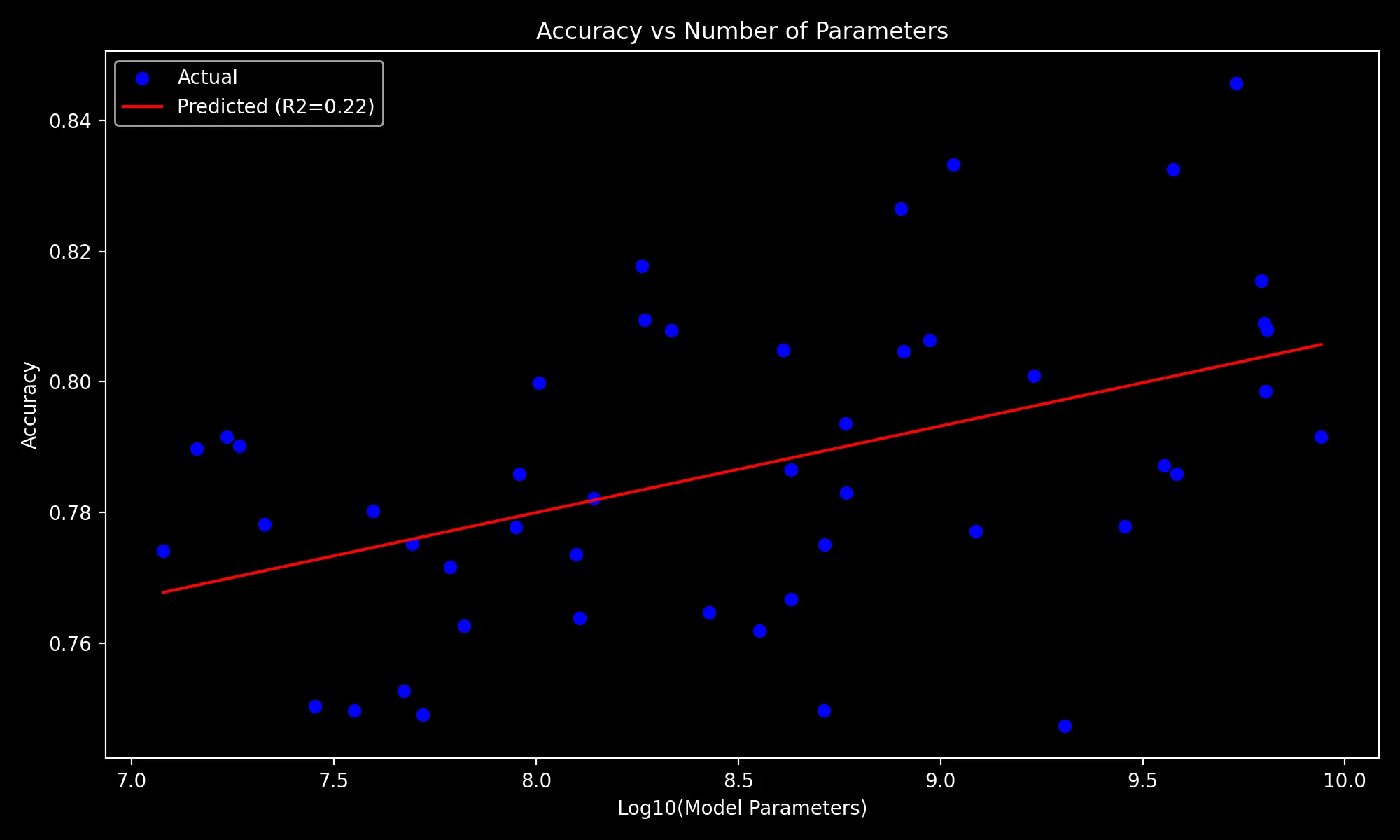
Scenario 2: Understanding AGI Timeline Predictions: A Chi-Square Analysis of Academia vs Industry
Research into AGI has sparked debates about when we might achieve this technological milestone. One interesting question is whether researchers’ work environments influence their predictions about AGI timelines. Let’s use this scenario as a case study for a chi-square analysis.
The Research Question
Do academic and industry researchers differ in their predictions about AGI timelines? This is a categorical variable, making it suitable for a chi-square test. Suppose we surveyed 400 AI researchers (200 from academia and 200 from industry) about when they expect AGI to be achieved. The responses were categorized as follows:
- < 2 years
- 2-5 years
- 5-10 years
- 10 years or more
Understanding Chi-Square Analysis
The chi-square test of independence helps us determine whether there’s a significant relationship between two categorical variables. It compares the observed frequencies of categories with the frequencies we would expect if the variables were independent. In our case, the variables are:
- Work Environment (Academia vs. Industry)
- AGI Timeline Prediction (four timeline categories)
The test works by comparing the observed frequencies in a contingency table with the frequencies we would expect if the variables were independent. Let’s create some sample data to illustrate this:
# Create example dataset representing a survey of AI researchers
np.random.seed(42)

# Generate sample data
n_researchers = 400  # Total number of surveyed researchers

# Create slightly different distribution of predictions for industry vs academia
# to demonstrate potential relationships
academia_predictions = np.random.choice(
    ['<10 years', '10-20 years', '20-50 years', '>50 years'],
    size=200,
    p=[0.15, 0.25, 0.35, 0.25]  # Academia tends toward longer timelines
)

industry_predictions = np.random.choice(
    ['<10 years', '10-20 years', '20-50 years', '>50 years'],
    size=200,
    p=[0.25, 0.35, 0.25, 0.15]  # Industry tends toward shorter timelines
)
The test statistic is calculated as:
where:
- is the observed frequency
- is the expected frequency
- The sum is taken over all cells in the contingency table
- The degrees of freedom (dof) is , where is the number of rows and is the number of columns.
To calculate the expected frequency for any cell, we use this formula:
Effect Size with Cramér’s V
Cramér’s V is a measure of association between two categorical variables. It’s based on the chi-square statistic and ranges from 0 to 1, where:
- 0 indicates no association
- 1 indicates a perfect association
The formula for Cramér’s V is:
where:
- is the chi-square statistic
- is the total number of observations
- and are the number of rows and columns in the contingency table
Performing the Chi-Square Test
We can carry this out in python by first creating a contingency table of observed frequencies and then calculating the chi-square statistic:
from collections import Counter

academic_counts = Counter(academia_predictions)
industry_counts = Counter(industry_predictions)

print("Academia AGI Counts:", academic_counts)
print("Industry AGI Counts:", industry_counts)

test_table = np.array(
    [
        [academic_counts[k] for k in agi_timelines],
        [industry_counts[k] for k in agi_timelines],
    ]
)
print(test_table)
>>>
Academia AGI Counts: Counter({'5-10 years': 59, '2-5 years': 57, '>10 years': 51, '<2 years': 33})
Industry AGI Counts: Counter({'2-5 years': 64, '5-10 years': 57, '<2 years': 49, '>10 years': 30})
[[33 57 59 51]
 [49 64 57 30]]
Then we can calculate the chi-square statistic and Cramer’s V:
import numpy as np
from scipy import stats


def chi2_test(contingency_table: np.ndarray | list[list[int]]) -> dict:
    observed = np.array(contingency_table)

    row_totals = observed.sum(axis=1)
    col_totals = observed.sum(axis=0)
    total = row_totals.sum()

    # E_ij = (row_total_i * col_total_j) / grand_total
    expected = np.outer(row_totals, col_totals) / total

    chi2 = np.sum((observed - expected) ** 2 / expected)
    dof = (observed.shape[1] - 1) * (observed.shape[0] - 1)

    p_value = 1 - stats.chi2.cdf(chi2, dof)

    min_dim = min(observed.shape) - 1
    cramers_v = np.sqrt(chi2 / (total * min_dim))
    std_residuals = (observed - expected) / np.sqrt(expected)

    return {
        "ch2": chi2,
        "expected": expected,
        "dof": dof,
        "p_value": p_value,
        "cramers_v": cramers_v,
        "std_residuals": std_residuals,
    }
import pandas as pd
work_env = ['Academia'] _ 200 + ['Industry'] _ 200
agi_timelines = ['<2 years', '2-5 years', '5-10 years', '>10 years']
df = pd.DataFrame({
'Work Environment': work_env,
'AGI Timeline': np.concatenate([academia_predictions, industry_predictions])
})
contingency_table = pd.crosstab(df['Work Environment'], df['AGI Timeline'])
percentages = (
pd.crosstab(
data["Work_Environment"],
data["AGI_Timeline"],
normalize="index",
)
* 100
)
# Perform chi-square test
chi2, p_value, dof, expected = chi2_contingency(contingency_table)Interpreting the Results
The test gives the following results:
Analysis of AGI Timeline Predictions Across Research Environments
-------------------------------------------------------------

1. Distribution of Predictions:
AGI_Timeline      2-5 years  5-10 years  <2 years  >10 years  All
Work_Environment
Academia                 57          59        33         51  200
Industry                 64          57        49         30  200
All                     121         116        82         81  400

2. Percentage Distribution within Each Environment:
AGI_Timeline      2-5 years  5-10 years  <2 years  >10 years
Work_Environment
Academia               28.5        29.5      16.5       25.5
Industry               32.0        28.5      24.5       15.0

3. Statistical Test Results:
Chi-squared statistic: 9.01
p-value: 0.0292
Degrees of freedom: 3
Cramer's V (effect size): 0.150
The contingency table show some interesting patterns:
- In Academia: The highest proportion (29.5%) predict AGI in 5-10 years
- In Industry: The highest proportion (32.0%) predict AGI in 2-5 years
- Notable difference: 25.5% of academics predict >10 years compared to only 15.0% of industry researchers
Since our p-value (0.0292) is less than the conventional significance level of 0.05, we can conclude that there is a statistically significant relationship between work environment and AGI timeline predictions.
Key Takeaways
- There is a statistically significant relationship between work environment and AGI timeline predictions .
- Industry researchers tend to predict shorter timelines compared to academic researchers.
- The relationship, while significant, is moderate in strength (Cramer’s V = 0.150).
- The most notable differences appear in the extreme categories ( years and >50 years).