Training neural networks at truly large-scale is not easy. Training frontier models like GPT-4o and Claude-3.5-sonnet demanded immense computational resources - in fact, very few are fortunate enough to train on thousands of H100s, but it is an interesting challenge and one that is critically important for modern AI. In this post, we will explore a sequence of increasingly sophisticated techniques for training neural networks at scale, from standard distributed data parallelism to Fully Sharded Data Parallelism with pipelining. We will also discuss the challenges of training large-scale models and how to address them.
*This post is motivated by srush’s LLM-Training-Puzzles.
Table of Contents
Open Table of Contents
Introduction
Anatomy of a Neural Network Training Loop
Let’s start by examining the traditional training loop. At its core, a neural network training loop involves:
- Forward Pass: Computing predictions and loss for a batch of data.
- Backward Pass: Computing gradients by backpropagation.
- Optimization Step: Applying gradients to update model weights.
In its simplest form, the training loop looks like this:
model = Model()
optimizer = Optimizer(model.parameters(), lr=0.001)
criterion = LossFunction()

for epoch in range(num_epochs):
    for data, targets in data_loader:
        # Forward pass
        outputs = model(data)
        loss = criterion(output, targets)

        # Backward pass
        optimizer.zero_grad()
        loss.backward()

        # Optimization step
        optimizer.step()
We’ve seen this loop many times before, but what happens when we scale it up to train on thousands of GPUs? The training loop becomes more complex, with additional challenges and opportunities at each phase.
Mixed Precision Training
Mixed precision training is a technique that combines different numerical precisions in a single model to improve performance and reduce memory usage without sacrificing model accuracy. This approach is particularly useful for large-scale training, as it allows for faster computation and reduced memory footprint.
Key Concepts of Mixed Precision Training
-
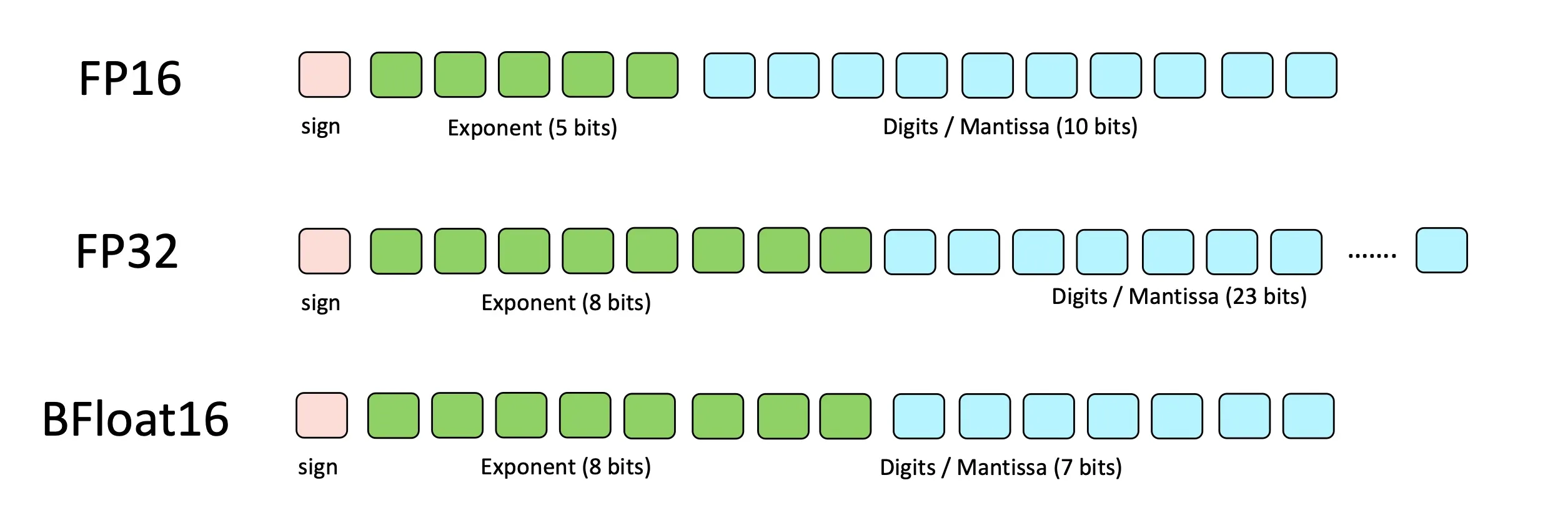
FP32 (single-precision) vs FP16 (half-precision): FP32 uses 32 bits to represent a number, while FP16 uses 16 bits. FP16 requires less memory and enables faster computation, but has a smaller range and less precision.
-
Master weights in FP32: The model’s master weights are kept in FP32 for stability and accuracy.
-
Forward and backward passes in FP16: Computations in the forward and backward passes are performed in FP16 for speed.
-
Loss scaling: To prevent underflow in gradients, the loss is scaled up before backpropagation and gradients are scaled down before updating weights. Update the master weights in FP32.
-
Dynamic loss scaling: The scaling factor is adjusted dynamically based on whether gradient overflow occurs.
To recap, typically during training we store the following in GPU VRAM:
NN:
- Model parameters (in FP16)
- Forward pass activations (FP16)
- Backward pass gradients (FP16)
Optimizer:
- Master weights (FP32)
- Adam momentum (FP32)
- Adam variance (FP32)
Implementation with PyTorch
PyTorch provides built-in support for mixed precision training through its torch.cuda.amp module. Here’s a basic example of how to modify our training loop to use mixed precision:
import torch
from torch.cuda.amp import GradScaler

device = torch.device("cuda" if torch.cuda.is_available() else "cpu")

model = Model().to(device)
criterion = torch.nn.CrossEntropyLoss()
optimizer = torch.optim.Adam(model.parameters(), lr=0.001)
scaler = GradScaler()
use_amp = True  # Set to False to disable mixed precision

for epoch in range(num_epochs):
    for data, targets in data_loader:
        data, targets = data.cuda(), targets.cuda()

        # Forward pass with autocasting
        with torch.autocast(device_type=device, dtype=torch.float16, enabled=use_amp):
            outputs = model(data)
            loss = criterion(outputs, targets)

        # Backward pass with scaled gradients
        optimizer.zero_grad()
        # Scales loss. Calls ``backward()`` on scaled loss to create scaled gradients.
        scaler.scale(loss).backward()

        # If these gradients do not contain ``inf``s or ``NaN``s, optimizer.step() is then called,
        # otherwise, optimizer.step() is skipped
        scaler.step(optimizer)

        # Updates the scale for next iteration.
        scaler.update()
In this example, autocast() enables automatic mixed precision for the forward pass, while GradScaler handles loss scaling for the backward pass.
Gradient scaling helps prevent gradients with small magnitudes from flushing to zero (“underflowing”) when training with mixed precision. It is a crucial step in ensuring the stability and convergence of the training process.
Greater Dynamic Range with Bfloat16
The reason we need loss/gradient scaling in mixed precision training is that FP16 has a smaller range and less precision than FP32. To address this, a new numerical format called bfloat16 (BF16) has been introduced. BF16 offers a larger dynamic range than FP16 while maintaining the speed benefits of reduced precision. It does so by allocating 8 bits for the exponent and 7 bits for the mantissa, providing a wider range of representable values.
Collective Communication Operations
Collective operations are building blocks for interaction patterns in distributed computing. They are used to move and synchronize data across multiple devices, such as GPUs, in a distributed system.
To understand collective operations quickly, I believe pictures are worth a thousand words. Here are some visualizations of common collective operations:
Notation:
- Rank: We’ll denote rank by where ranges from 1 to .
- Local Data Vectors: Each rank holds a local data vector .
- Concatenated Vector: The concatenated result of gathering local data vectors is .
- Operation Result: For reductions, the result of an operation (e.g., sum) will be denoted by .
- Scatter Result: Given a data array , Scatter sends to rank .
In code: We’ll also go through the equivalent PyTorch code for each operation. In order to run these operations, you’ll need to set up a distributed environment. Here’s a simple utility function to run distributed functions in PyTorch:
def init_process(
    rank: int, world_size: int, fn: Callable[[int, int], None], backend="gloo"
):
    """Initialize the distributed environment for a process and run the function."""
    os.environ["MASTER_ADDR"] = "127.0.0.1"
    os.environ["MASTER_PORT"] = "29500"
    dist.init_process_group(backend, rank=rank, world_size=world_size)
    fn(rank, world_size)


def run_dist_fn(fn: Callable[[int, int], None], num_ranks: int = 4):
    """Run a distributed function with the specified number of ranks."""
    print(f"Running {fn.__name__} with {num_ranks} processes")
    processes = []
    try:
        mp.set_start_method("spawn")
    except RuntimeError:
        pass
    for rank in range(num_ranks):
        p = mp.Process(target=init_process, args=(rank, num_ranks, fn))
        p.start()
        processes.append(p)

    for p in processes:
        p.join()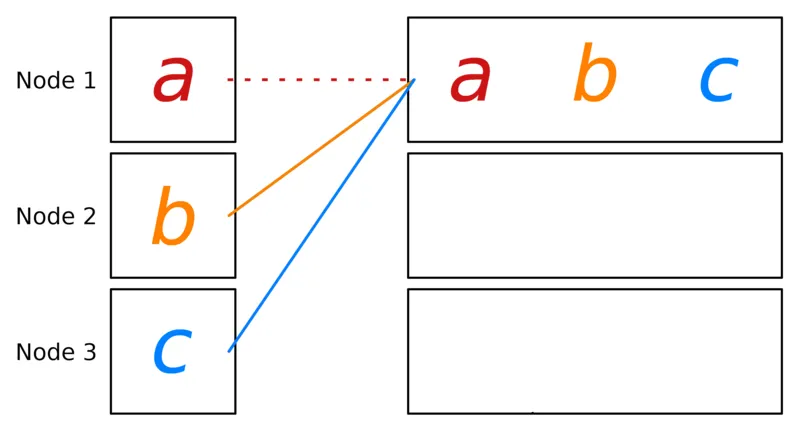
def do_gather(rank: int, size: int):
  # create a group with all processors
  group = dist.new_group(list(range(size)))
  # create a tensor with the rank number
  input_tensor = torch.tensor([rank], dtype=torch.float32)

  if rank == 0:
      # gathering from all ranks
      # create an empty list we will use to hold the gathered values
      glist = [torch.empty(1) for _ in range(size)]
      dist.gather(input_tensor, gather_list=glist, dst=0, group=group)
  else:
      # sending tensor to rank 0
      dist.gather(input_tensor, dst=0, group=group)

  if rank == 0:
      # only rank 0 will have the tensors from the other processed
      # [tensor([0.]), tensor([1.]), tensor([2.]), tensor([3.])]
      print(f"[{rank}] data = {torch.cat(glist)}")
The Gather operation collects data from multiple ranks into a single rank. Gather merges them into a concatenated vector .
def do_all_gather(rank: int, size: int):
# create a group with all processors
group = dist.new_group(list(range(size)))
tensor = torch.tensor([rank], dtype=torch.float32)
# create an empty list we will use to hold the gathered values
tensor_list = [torch.empty(1) for _ in range(size)]
# sending all tensors to the others
dist.all_gather(tensor_list, tensor, group=group)
# all ranks will have
# [tensor([0.]), tensor([1.]), tensor([2.]), tensor([3.])]
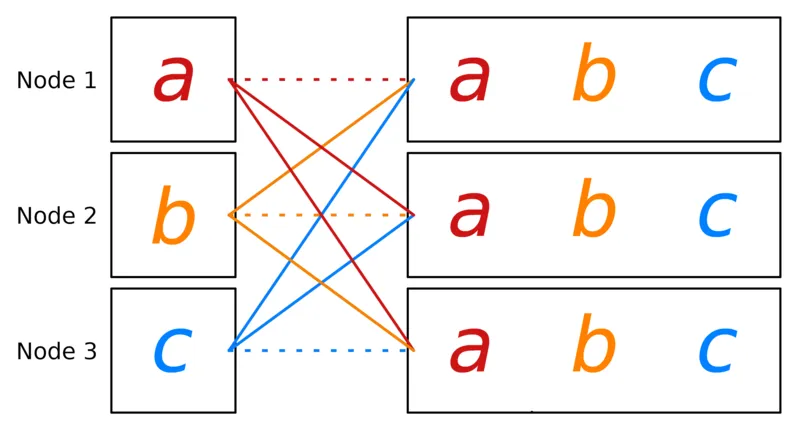
print(f"[{rank}] data = {tensor_list}")All Gather extends Gather by distributing the concatenated vector to all ranks. Thus, each rank ends up with a copy of .
def do_broadcast(rank: int, size: int):
# create a group with all processors
group = dist.new_group(list(range(size)))
if rank == 0:
tensor = torch.tensor([rank], dtype=torch.float32)
else:
tensor = torch.empty(1)
# sending all tensors to the others
dist.broadcast(tensor, src=0, group=group)
# all ranks will have tensor([0.]) from rank 0
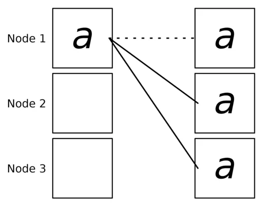
print(f"[{rank}] data = {tensor}")Broadcast sends data from one rank to all others. If rank holds the data , Broadcast ensures all ranks receive .
def do_scatter(rank: int, size: int):
# create a group with all processors
group = dist.new_group(list(range(size)))
# Tensor memory for all ranks
out_tensor = torch.empty(1)
# sending all tensors from rank 0 to the others
if rank == 0:
# only rank 0 sends out the data
slist = [
torch.tensor([i + 1], dtype=torch.float32)
for i in range(size)
]
# slist = [tensor(1), tensor(2), tensor(3), tensor(4)]
dist.scatter(out_tensor, scatter_list=slist, src=0, group=group)
else:
dist.scatter(out_tensor, scatter_list=[], src=0, group=group)
# each rank will have a tensor with their rank number
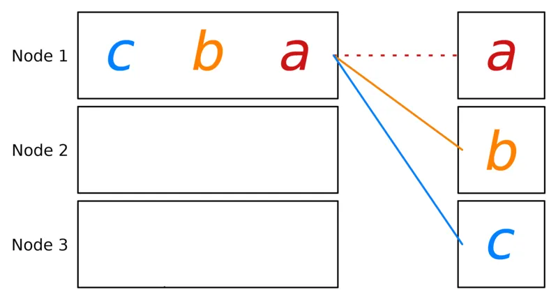
print(f"[{rank}] data = {out_tensor[0]}")Scatter distributes parts of a data array to different ranks. Given a data array , Scatter sends to rank .
def do_reduce(rank: int, size: int):
# create a group with all processors
group = dist.new_group(list(range(size)))
tensor = torch.ones(1)
# sending all tensors to rank 0 and sum them
# Interestingly, other ranks will have intermediate values
dist.reduce(tensor, dst=0, op=dist.ReduceOp.SUM, group=group)
# can be dist.ReduceOp.PRODUCT, dist.ReduceOp.MAX, dist.ReduceOp.MIN
# only rank 0 will have four
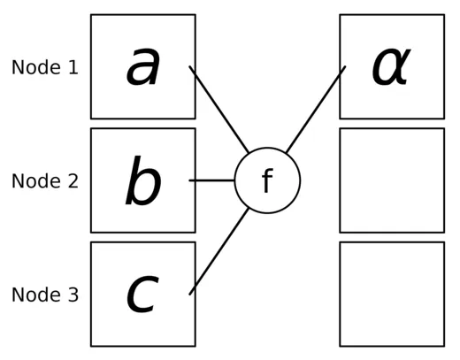
print(f"[{rank}] data = {tensor[0]}")Reduce aggregates data from all ranks using a specified operation (e.g., sum, max). For summation, the result is sent to a particular rank.
def do_all_reduce(rank: int, size: int):
# create a group with all processors
group = dist.new_group(list(range(size)))
tensor = torch.ones(1)
dist.all_reduce(tensor, op=dist.ReduceOp.SUM, group=group)
# can be dist.ReduceOp.PRODUCT, dist.ReduceOp.MAX, dist.ReduceOp.MIN
# will output 4 for all ranks
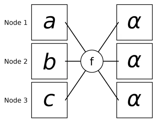
print(f"[{rank}] data = {tensor[0]}")AllReduce performs a Reduce followed by a Broadcast, providing all ranks with the same aggregated result .
def reduce_scatter(rank: int, size: int):
group = dist.new_group(list(range(size)))
tensor = torch.ones(1).to(rank)
input_tensor = [
(i + 1) * torch.tensor([1 + rank], device=f"cuda:{rank}")
for i in range(size)
]
print(f"[{rank}] input_tensor = {input_tensor}")
dist.reduce_scatter(
tensor,
input_tensor,
op=dist.ReduceOp.SUM,
group=group,
)
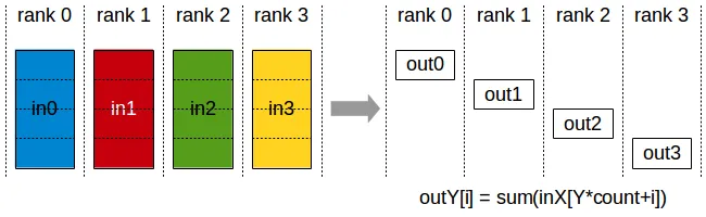
print(f"[{rank}] data = {tensor[0]}")ReduceScatter combines Reduce and Scatter: input values are reduced across ranks, with each rank receiving a subpart of the result. is split into equal blocks, where is sent to rank .
Distributed Data Parallelism
Distributed Data Parallelism (DDP) is a fundamental technique for scaling neural network training across multiple devices. In this approach, the model is replicated across multiple devices, and each device processes a different subset of the data.
How DDP Works
- Model Replication: The entire model is copied to each device (e.g., GPU).
- Data Distribution: The training data is divided into batches and distributed across devices.
- Forward Pass: Each device performs a forward pass on its local data batch.
- Backward Pass: Each device computes gradients based on its local data.
- Gradient Synchronization: Gradients from all devices are aggregated using an
all_reduceoperation. - Parameter Update: Each device updates its local copy of the model using the synchronized gradients.
Communication Pattern: all_reduce to synchronize gradients across devices.
Implementation with PyTorch
Here’s a basic example of how to implement DDP using PyTorch:
import os

import torch
import torch.distributed as dist
import torch.multiprocessing
import torch.nn as nn
from torch.nn.parallel import DistributedDataParallel as DDP


def setup(rank, world_size):
    os.environ["MASTER_ADDR"] = "127.0.0.1"
    os.environ["MASTER_PORT"] = "29500"
    dist.init_process_group("nccl", rank=rank, world_size=world_size)


class ToyModel(nn.Module):
    def __init__(self):
        super().__init__()
        self.net1 = nn.Linear(10, 10)
        self.relu = nn.ReLU()
        self.net2 = nn.Linear(10, 5)

    def forward(self, x):
        return self.net2(self.relu(self.net1(x)))


def dataloader():
    for _ in range(100):
        data = torch.randn(10, 10)
        target = torch.randint(0, 5, (10,))
        yield data, target


def train(rank, world_size):
    setup(rank, world_size)

    model = ToyModel().to(rank)
    ddp_model = DDP(model, device_ids=[rank])
    criterion = nn.CrossEntropyLoss()

    optimizer = torch.optim.Adam(ddp_model.parameters(), lr=0.001)

    for epoch in range(2):
        for data, target in dataloader():
            data, target = data.to(rank), target.to(rank)
            optimizer.zero_grad()
            output = ddp_model(data)
            loss = criterion(output, target)
            loss.backward()
            optimizer.step()
        print(f"Rank {rank} / {world_size} / {epoch}: loss {loss.item()}")


if __name__ == "__main__":
    world_size = torch.cuda.device_count()
    torch.multiprocessing.spawn(train, args=(world_size,), nprocs=world_size)
'''
Pros and Cons
Advantages of DDP
- Simplicity: Relatively easy to implement as the model architecture remains unchanged.
- Scalability: Can efficiently utilize multiple GPUs or even multiple machines.
- Load Balancing: Computational workload is evenly distributed across devices.
- Memory Efficiency: Each device only needs to store one copy of the model and its data batch.
Challenges of DDP
- Communication Overhead: The
all_reduceoperation can be expensive, especially with slow network connections between devices. - Batch Size Considerations: The effective batch size increases with the number of devices, which may affect model convergence.
- Limited by Model Size: Each device must be able to hold the entire model, which can be a limitation for very large models.
Model (Weight-sharded) Parallelism
Model Parallelism, also known as Weight-sharded Parallelism, is a technique that partitions the model parameters across multiple devices. This approach is particularly useful when the model is too large to fit on a single device.
How Model Parallelism Works
- Model Partitioning: The model’s layers or parameters are divided among multiple devices.
- Forward Pass:
- Input data is passed through the first partition on one device.
- Output is transferred to the next device for processing through the next partition.
- This continues until the final output is produced.
- Backward Pass:
- Gradients are computed in reverse order through the partitioned model.
- Each device computes gradients for its portion of the model.
- Parameter Update: Each device updates its local portion of the model parameters.
Types of Model Parallelism
There are two primary types of model parallelism. They have slightly different communication patterns and trade-offs:
- Layer-wise Parallelism: Different layers of the model are assigned to different devices.
- E.g., Layer 1 on GPU 1, Layer 2 on GPU 2, etc.
- Requires an
all_reduceto synchronize gradients before weight update (like DDP)
- Tensor Parallelism: Individual tensors (e.g., weight matrices) are split across devices.
- E.g., First half of the weight matrix on GPU 1, second half on GPU 2.
- Requires reconstructing each layer with an
all_gatheroperation, then uses anall_reduceto synchronize gradients and update local weights.
Implementation Example - Layerwise Model Parallelism
Here’s a simplified example of layer-wise model parallelism using PyTorch:
class ToyMpModel(nn.Module):
    def __init__(self, dev0, dev1):
        super().__init__()
        self.dev0 = dev0
        self.dev1 = dev1
        self.net1 = torch.nn.Linear(10, 10).to(dev0)
        self.relu = torch.nn.ReLU()
        self.net2 = torch.nn.Linear(10, 5).to(dev1)

    def forward(self, x):
        # first device
        x = x.to(self.dev0)
        x = self.relu(self.net1(x))
        # second device
        x = x.to(self.dev1)
        return self.net2(x)
from torchvision.models.resnet import Bottleneck, ResNet
num_classes = 1000
class ModelParallelResNet50(ResNet):
def __init__(self, dev1: str, dev2: str | None = None, *args, **kwargs):
super(ModelParallelResNet50, self).__init__(
Bottleneck, [3, 4, 6, 3], num_classes=num_classes, *args, **kwargs
)
self.dev1 = dev1
self.seq1 = nn.Sequential(
self.conv1,
self.bn1,
self.relu,
self.maxpool,
self.layer1,
self.layer2,
).to(dev1)
self.dev2 = dev2 if dev2 is not None else dev1
self.seq2 = nn.Sequential(self.layer3, self.layer4, self.avgpool).to(self.dev2)
self.fc.to(self.dev2)
def forward(self, x: torch.Tensor):
x = self.seq2(self.seq1(x).to(self.dev2))
return self.fc(x.view(x.size(0), -1))Implementation Example - Tensor Parallelism
Here’s an example of tensor parallelism using PyTorch. In this example, we split the weight matrix of a linear layer across multiple devices:
import os

import torch
import torch.distributed as dist
import torch.multiprocessing as mp
import torch.nn as nn


class TensorParallelLinear(nn.Module):
    def __init__(self, in_features, out_features, world_size: int | None = None):
        super().__init__()
        self.in_features = in_features
        self.out_features = out_features
        if world_size is None:
            world_size = dist.get_world_size()
        self.world_size = world_size

        # Split the weight matrix along the output dimension
        self.out_features_per_rank = out_features // world_size
        self.weight = nn.Parameter(torch.randn(self.out_features_per_rank, in_features))
        self.bias = nn.Parameter(torch.randn(self.out_features_per_rank))

    def forward(self, input):
        # Perform local matrix multiplication
        local_output = torch.matmul(input, self.weight.t()) + self.bias

        # Gather results from all ranks
        gathered_output = [
            torch.zeros_like(local_output) for _ in range(self.world_size)
        ]
        dist.all_gather(gathered_output, local_output)

        # Concatenate the gathered results
        return torch.cat(gathered_output, dim=-1)


def setup(rank, world_size):
    os.environ["MASTER_ADDR"] = "localhost"
    os.environ["MASTER_PORT"] = "12356"
    dist.init_process_group("gloo", rank=rank, world_size=world_size)


def cleanup():
    dist.destroy_process_group()


def run_tensor_parallel(rank, world_size):
    print(f"Running on rank {rank}.")
    setup(rank, world_size)

    torch.manual_seed(42 + rank)
    model = TensorParallelLinear(1000, 1000, None).to(rank)
    input = torch.randn(32, 1000).to(rank)

    output = model(input)
    print(f"Rank {rank}: Output shape: {output.shape}")
    # Expected output:
    # Rank 0: Output shape: torch.Size([32, 1000])
    # Rank 1: Output shape: torch.Size([32, 2000])
    # Each rank computes a local output of shape (32, 500) and then gathers the results from all ranks.

    cleanup()


if __name__ == "__main__":
    world_size = 2
    mp.spawn(run_tensor_parallel, args=(world_size,), nprocs=world_size, join=True)
Use Cases:
- Large Models: Ideal when a single model is too large to fit into the memory of a single device.
- Sequential Computation: Best suited for models where layers can be neatly partitioned without significant inter-layer communication.
Pros and Cons
Advantages of Model Parallelism
- Memory Efficiency: Allows training of models that are too large to fit on a single device.
- Flexibility: Can be combined with data and pipeline parallelism for more efficient scaling.
Challenges of Model Parallelism
- Complex Implementation: Requires careful design of the model architecture and data flow.
- Potential for Idle Resources: Some devices may be underutilized if the workload is not balanced.
- Increased Latency: Sequential processing through partitions can increase the overall computation time.
- Limited by Inter-device Bandwidth: Performance can be bottlenecked by the speed of data transfer between devices.
Combining Model Parallelism with PyTorch DDP
DDP also works with multi-GPU models. DDP wrapping multi-GPU models is especially helpful when training large models with a huge amount of data. Check out the modified example below to see how to handle this. Note that each process will control 2 GPUs that house the model split across them.
# ... (Existing imports and code)

def train(rank, world_size):
    setup(rank, world_size)

    # Each process uses 2 GPUs
    dev0 = rank * 2
    dev1 = rank * 2 + 1
    mp_model = ToyMpModel(dev0, dev1)
    ddp_mp_model = DDP(mp_model)  # Don't pass device_ids to DDP
    criterion = nn.CrossEntropyLoss()

    optimizer = torch.optim.Adam(ddp_mp_model.parameters(), lr=0.001)

    for epoch in range(2):
        for data, target in dataloader():
            optimizer.zero_grad()
            # Let DDP handle moving the input data to the correct device
            output = ddp_mp_model(data)
            loss = criterion(output, target.to(output.device))
            loss.backward()
            optimizer.step()
            print(f"Rank {rank} / {world_size} / {epoch}: loss {loss.item()}")


if __name__ == "__main__":
    n_gpus = torch.cuda.device_count()
    assert n_gpus >= 2, f"Requires at least 2 GPUs to run, but got {n_gpus}"

    # Each process uses 2 GPUs
    world_size = n_gpus
    world_size = n_gpus // 2
    torch.multiprocessing.spawn(train, args=(world_size,), nprocs=world_size)
'''
Fully Sharded Data Parallelism
FSDP Workflow
Initialization:
- Shard model parameters so that each rank maintains its own shard of the model.
Forward Pass:
- For each FSDP Unit, run
all_gatherto collect all model parameters for this unit from other ranks - Run forward computation
- Discard parameter shards it has just collected
Backward Pass:
- Run
all_gatherto collect all parameter shards from other ranks in FSDP unit - Run backward computation (compute gradients)
- Perform
reduce_scatterto average and shard local gradients across the GPUs in the unit. Each GPU receives only the gradients needed to update its local weight shard. - Discard parameters
What’s the difference between FSDP and MP?
Model Parallelism (MP) and Fully Sharded Data Parallelism (FSDP) are different approaches to distributing model training across multiple devices:
- Model Partitioning vs. Parameter Sharding:
- Model Parallelism: Partitions the model layers or operations across devices.
- FSDP: Shards individual parameters and optimizer states across devices.
- Data Handling:
- Model Parallelism: The same data sample moves through different parts of the model on different devices.
- FSDP: Different devices process different data samples (mini-batches) independently but share sharded parameters.
- Memory Efficiency:
- Model Parallelism: Distributes model memory across devices but doesn’t reduce overall memory footprint.
- FSDP: Reduces per-device memory usage by sharding parameters and states, allowing larger models to be trained.
- Communication Patterns:
- Model Parallelism: Requires communication of activations and gradients between devices sequentially.
- FSDP: Involves all-gather operations to collect parameter and reduce-scatter operations to distribute gradients.
- Scalability:
- Model Parallelism: Limited by the number of partitions the model can be broken into effectively.
- FSDP: More scalable as adding more devices can reduce per-device memory load without significant model restructuring.
When to Use Which
Use Model Parallelism When:
- The model cannot fit into the memory of a single device, and partitioning the model is feasible.
- The model architecture allows for straightforward partitioning with minimal inter-partition communication.
Use FSDP When:
- Training extremely large models that exceed memory capacities even after considering model parallelism.
- You require the efficiency of data parallelism but need to mitigate the memory overhead of parameter replication.
Pipeline Parallelism
Pipeline parallelism partitions the layers of a model into stages where each stage is processed by a different device. As activations flow through the model, the outputs of one stage are communicated as inputs to the next stage. Once the forward pass is complete, the gradients are passed back through the pipeline stages, locally updating the model weights at each stage.
Sometimes called the “GPipe Schedule”, a batch of data can be split into “micro-batches” that are processed in parallel by the pipeline stages. Once a stage completes a forward pass for a micro-batch, the activations are passed to the next stage in the pipeline. Similarly, gradients are passed back through the pipeline stages. Each backward pass utilizes local gradient accumulation to calculate the gradients for the entire batch. If data parallelism is used in conjunction with pipeline parallelism (see below), data-parallel groups reduce the gradients in parallel before updating the model weights.
Pipeline parallelism can be combined with data parallelism (or even model parallelism) to vastly increase the size of models that can be trained. For example, Deepspeed + Megatron-LM uses this 3D parallelism to train models with trillions of parameters.
How Pipeline Parallelism Works
- Model Partitioning: The model is divided into sequential stages.
- Micro-batch Processing: Input data is split into micro-batches.
- Forward Pass: Micro-batches flow through the pipeline, with each stage processing and passing results to the next.
- Backward Pass: Gradients flow backwards through the pipeline.
- Gradient Accumulation: Gradients are accumulated locally at each stage.
- Parameter Update: After processing all micro-batches, each stage updates its parameters.
Implementation Example
Manual (hardcoded layerwise pipeline parallelism)
To understand the basic concept of pipeline parallelism, consider the toy example below where we manually define the stages of the pipeline. In the forward pass, we explicitly pass the output of one stage to the next stage. In practice, more sophisticated scheduling mechanisms are used to automate this process.
class ToyPipelineParallelPMpModel(nn.Module):
    def __init__(self, dev0, dev1, split_size: int = 32):
        super().__init__()
        self.dev0 = dev0
        self.dev1 = dev1
        self.net1 = torch.nn.Linear(10, 10).to(dev0)
        self.relu = torch.nn.ReLU()
        self.net2 = torch.nn.Linear(10, 5).to(dev1)
        self.split_size = split_size

    # Define the stages of the pipeline

    def stage1(self, x: torch.Tensor):
        x = x.to(self.dev0)
        x = self.relu(self.net1(x))
        return x

    def stage2(self, x: torch.Tensor):
        x = x.to(self.dev1)
        return self.net2(x)

    def forward(self, x: torch.Tensor):
        # Split the input into micro-batches

        splits = iter(x.split(self.split_size, dim=0))
        s1_input = next(splits)

        # Prefill the first stage
        s2_input = self.stage1(s1_input)

        out = []
        for s1_input in splits:
            out.append(self.stage2(s2_input))
            s2_input = self.stage1(s1_input)

        # Process the last micro-batch
        s2_out = self.stage2(s2_input)
        out.append(s2_out)
        return torch.cat(out)
In practice, you may encountered higher-level abstractions for pipeline parallelism, where frameworks may provide wrapper classes that attempt to automate the process of defining and executing pipeline stages.
import torch
import torch.nn as nn


class PipelineStage(nn.Module):
    def __init__(self, layers, device):
        super().__init__()
        self.layers = nn.Sequential(*layers).to(device)
        self.device = device

    def forward(self, x):
        return self.layers(x.to(self.device))


class PipelineParallelModel(nn.Module):
    def __init__(self, num_stages):
        super().__init__()
        self.stages = nn.ModuleList(
            [
                PipelineStage([nn.Linear(1000, 1000), nn.ReLU()], f"cuda:{i}")
                for i in range(num_stages)
            ]
        )
        self.output_layer = nn.Linear(1000, 10).to(f"cuda:{num_stages-1}")

    def forward(self, x):
        for stage in self.stages:
            x = stage(x)
        return self.output_layer(x)


def train_pipeline_parallel(model, data, num_micro_batches):
    optimizer = torch.optim.Adam(model.parameters())
    criterion = nn.CrossEntropyLoss()

    for epoch in range(10):
        for batch, targets in data:
            micro_batches = torch.chunk(batch, num_micro_batches)
            micro_targets = torch.chunk(targets, num_micro_batches)

            # Forward pass
            outputs = []
            for micro_batch in micro_batches:
                output = model(micro_batch)
                outputs.append(output)

            # Backward pass
            optimizer.zero_grad()
            for i, output in enumerate(reversed(outputs)):
                target = micro_targets[num_micro_batches - i - 1]
                loss = criterion(output, target.to(output.device))
                loss.backward()

            optimizer.step()
            print(loss.item())


def dataloader():
    for _ in range(100):
        yield torch.randn(10, 1000), torch.randint(0, 10, (10,))


model = PipelineParallelModel(num_stages=2)
train_pipeline_parallel(model, dataloader(), num_micro_batches=4)
This example demonstrates a basic implementation of pipeline parallelism. In practice, more sophisticated scheduling and synchronization mechanisms would be used to optimize performance.
FSDP with Pipelining
Combining Fully Sharded Data Parallelism (FSDP) with Pipeline Parallelism creates a powerful approach for training extremely large models efficiently. This combination allows us to leverage the memory efficiency of FSDP and the computational efficiency of pipeline parallelism.
How it Works
-
Model Partitioning: The model is first divided into pipeline stages, with each stage assigned to a different group of GPUs.
-
FSDP Within Stages: Within each pipeline stage, FSDP is applied to shard the parameters of that stage across the GPUs in that group.
-
Microbatch Processing: The input batch is divided into microbatches, which flow through the pipeline stages.
-
Forward Pass:
- Each stage performs its forward computation on a microbatch.
- FSDP handles the all-gather and sharding of parameters within the stage.
- Activations are passed to the next stage.
-
Backward Pass:
- Gradients flow backwards through the pipeline.
- FSDP handles the reduce-scatter of gradients within each stage.
-
Optimization: After processing all microbatches, each GPU updates its local parameter shard.
Benefits
- Reduced Memory Footprint: FSDP reduces the memory required per GPU by sharding parameters.
- Increased Parallelism: Pipeline parallelism allows for efficient utilization of multiple GPUs.
- Scalability: This approach can scale to very large models and cluster sizes.
Challenges
- Complex Implementation: Combining FSDP and pipeline parallelism requires careful orchestration of data movement and synchronization.
- Load Balancing: Ensuring even distribution of computation across pipeline stages and GPUs can be tricky.
- Communication Overhead: Managing the additional communication introduced by both FSDP and pipelining is crucial for performance.
Example Pseudocode
Here’s a high-level pseudocode to illustrate the concept:
def fsdp_pipeline_train(model, dataloader, num_stages, num_gpus_per_stage):
    # Partition model into pipeline stages
    stages = partition_model(model, num_stages)

    # Apply FSDP to each stage
    for stage in stages:
        stage = FSDP(stage, num_gpus_per_stage)

    for batch in dataloader:
        microbatches = split_batch(batch)

        for microbatch in microbatches:
            # Forward pass through pipeline
            for stage in stages:
                with stage.fsdp_context():
                    output = stage(microbatch)
                microbatch = output

            # Backward pass through pipeline
            for stage in reversed(stages):
                with stage.fsdp_context():
                    stage.backward(gradients)

        # Update parameters for each stage
        for stage in stages:
            stage.optimizer_step()
This pseudocode provides a simplified view of how FSDP and pipeline parallelism can be combined. In practice, the implementation would involve more complex synchronization and data management.
Low Rank Adaptation (LoRA)
Low Rank Adaptation (LoRA) is a parameter-efficient fine-tuning technique that significantly reduces the number of trainable parameters while maintaining model performance. This approach is particularly useful for adapting large pre-trained models to specific tasks with limited computational resources. It was introduced in this paper.
How LoRA Works
- Freezing Base Model: The parameters of the pre-trained model are kept frozen.
- Low-Rank Decomposition: Instead of fine-tuning all parameters, LoRA introduces small, trainable rank decomposition matrices to each weight matrix.
- Update Rule: During inference, the original weight matrix is updated as follows:
Where and are low-rank matrices with , and is the tradeoff between pre-trained “knowledge” and task-specific “knowledge.” Note: Only A and B contain trainable parameters. is the rank of the decomposition.
Implementation Example
Here’s a simplified implementation of LoRA in PyTorch:
import torch
import torch.nn as nn


class LoRALinear(nn.Module):
    def __init__(self, in_features, out_features, rank=4, alpha=16):
        super().__init__()
        self.rank = rank
        self.alpha = alpha
        self.scale = alpha / rank
        self.lora_B = nn.Parameter(torch.zeros(in_features, rank))
        self.lora_A = nn.Parameter(torch.zeros(rank, out_features))
        nn.init.kaiming_uniform_(self.lora_A, a=math.sqrt(5))
        nn.init.zeros_(self.lora_B)

    def forward(self, x):
        return x @ self.lora_B @ self.lora_A * self.scale


class LoRAModel(nn.Module):
    def __init__(self, base_model, rank=4):
        super().__init__()
        self.base_model = base_model
        self.lora_layers = nn.ModuleDict()

        for name, module in self.base_model.named_children():
            if isinstance(module, nn.Linear):
                self.lora_layers[name] = LoRALayer(
                    module.in_features, module.out_features, rank
                )

    def forward(self, x):
        """This assumes that the base model's children are named modules called in order."""
        for name, module in self.base_model.named_children():
            if isinstance(module, nn.Linear):
                lora_output = self.lora_layers[name](x)
                x = module(x) + lora_output
            else:
                x = module(x)
        return x

# Usage
base_model = ToyModel()
lora_model = LoRAModel(base_model, rank=4)

# Freeze base model parameters
for param in base_model.parameters():
    param.requires_grad = False

# Train only LoRA parameters
optimizer = torch.optim.Adam(lora_model.lora_layers.parameters(), lr=1e-3)
Advantages of LoRA
- Parameter Efficiency: Significantly reduces the number of trainable parameters.
- Memory Efficiency: Requires less memory during fine-tuning and inference.
- Fast Adaptation: Enables quick adaptation to new tasks or domains.
- Performance: Often achieves comparable performance to full fine-tuning.
Considerations
- The choice of rank affects the trade-off between model capacity and efficiency.
- LoRA is particularly effective for transformer-based models but can be applied to other architectures as well.
- While LoRA reduces the parameter count, it may introduce some computational overhead during inference.
Challenges and Future Directions
Training at scale involves significant challenges:
- Hardware Constraints: The computational and energy needs.
- Data Availability: Ensuring sufficient high-quality training data.
- Innovation needs: Advancements in algorithms and infrastructure to overcome limitations.
Future research may focus on improving energy efficiency and reducing computational demands through algorithmic innovations.
Conclusion
Efficient large-scale model training opens new avenues in AI applications. Implementing advanced parallelism and optimizing resource use offers immense advantages. Aspiring practitioners should experiment with these techniques on smaller scales, leveraging tools like PyTorch and TensorFlow.