Flash Attention in a Flash

Open Table of Contents

Jumping right In
Flash Attention is a Kernel Fusion Operation
Online Softmax “trick”
Algorithm 1: FlashAttention
Flash Attention Visualized

Jumping right In

Here, we will quickly go through the widely used Flash Attention mechanism [1] and understand why it’s such incredible algorithm for performing attention, and doing so very quickly.

TL;DR: It restructures how it computes the softmax for the attention matrix that is very mindful of the performance characteristics of modern GPU HBM (high bandwidth memory) and shared memory. It avoids materializing the $N \times N$ attention matrix, which is a very large matrix, and never reads or writes to the HBM. This is achieved by using an online softmax trick that allows for incremental evaluation of the softmax without realizing all the inputs to the softmax normalization.

First, consider the fairly standard PyTorch implementation for multi-head causal attention:

class CausalAttention(nn.Module):
    # ...(init method)...

    def forward(self, x: torch.Tensor):
        bsz, seqlen, dim = x.shape
        xq, xk, xv = self.wq(x), self.wk(x), self.wv(x)
        xq = xq.reshape(bsz, seqlen, self.num_heads_q, self.head_dim)
        xk = xk.reshape(bsz, seqlen, self.num_heads_kv, self.head_dim)
        xv = xv.reshape(bsz, seqlen, self.num_heads_kv, self.head_dim)

        xq = xq.transpose(1, 2)  # (bsz, num_heads_q, seqlen, head_dim)
        xk = xk.transpose(1, 2)  # (bsz, num_heads_kv, seqlen, head_dim)
        xv = xv.transpose(1, 2)  # (bsz, num_heads_kv, seqlen, head_dim)


        # Flash Attention modifies the following lines
        attn = (xq @ xk.transpose(-2, -1)) / (self.head_dim**0.5)
        attn = attn + self.mask[:, :, :seqlen, :seqlen]
        attn = F.softmax(attn, dim=-1)
        attn = self.attn_dropout(attn)
        out = attn @ xv

        # restore seqlen into batch dim and concatenate heado
        out = out.transpose(1, 2).contiguous().view(bsz, seqlen, -1)

        out = self.wo(out)

Now, focus your attetion on the highlighted lines above, and consider how data moves in and out of the high bandwidth memory (HBM) in a typical multi-head attention operation:

Require: Matrices $\mathbf{Q}, \mathbf{K}, \mathbf{V} \in \mathbb{R}^{N \times d}$ in HBM.

Load $\mathbf{Q}, \mathbf{K}$ by blocks from HBM, compute $\mathbf{S} = \mathbf{Q}\mathbf{K}^T$ , write $\mathbf{S}$ to HBM.
Read $\mathbf{S}$ from HBM, compute $\mathbf{P} = \text{softmax}(\mathbf{S})$ , write $\mathbf{P}$ to HBM.
Load $\mathbf{P}$ and $\mathbf{V}$ by blocks from HBM, compute $\mathbf{O} = \mathbf{P}\mathbf{V}$ , write $\mathbf{O}$ to HBM.
Return $\mathbf{O}$ .

What makes the above steps inefficient is that the $N \times N$ attention matrix $\mathbf{S}$ and $\mathbf{P}$ is materialized fully at each step, and reading/writing this huge matrix to HBM is very expensive. This is where all the queries and keys interact, and for each head, for each batch element, we’re getting a $T \times T$ matrix of attention, which is a million numbers, even for a single head, at a single batch index, like so.So basically this is a ton of memory, and this is never materialized.

Flash Attention comes into play by modifying these steps, implementing them very quickly. But how does it do that?

Flash Attention is a Kernel Fusion Operation

Well, flash attention is a kernel fusion operation. So you see here, on the right side of the diagram, they’re showing PyTorch and you have these five operations. And instead of those, we are fusing them into a single fused kernel of flash attention.

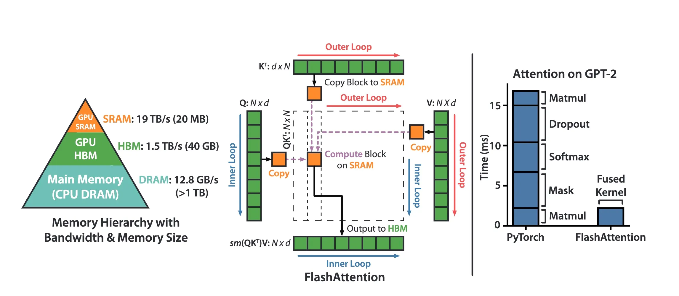
So it’s a kernel fusion algorithm, but it’s a kernel fusion that torch compile cannot find. And the reason that it cannot find it is that it requires an algorithmic rewrite of how attention is actually implemented here in this case. And what’s remarkable about it is that flash attention, actually, if you just count number of flops, flash attention does more flops than this attention here.

But flash attention is actually significantly faster. In fact, they cite 7.6 times faster, potentially. And that’s because it is very mindful of the memory hierarchy, as I mentioned. And so it’s very mindful about what’s in high bandwidth memory, what’s in the shared memory, and it is very careful without orchestras to computation, such that we have fewer reads and writes to the high bandwidth memory. And so even though we’re doing more flops, the expensive part is they’re load and store into HPM, and that’s what they avoid.

Online Softmax “trick”

How does Flash Attention avoid materializing the $N \times N$ attention matrix?

The way that this is achieved is that basically the fundamental algorithm agree right here relies on this online softmax trick, which was proposed previously [2]. The online softmax trick coming from a previous paper shows how you can incrementally evaluate a softmax without having to sort of realize all of the inputs to the softmax of the normalization. And remarkably, it came out of Nvidia. And it came out of it like really early 2018. So this is four years before Flash attention. And this paper says that,

We propose a way to compute the classical softmax with fewer memory accesses and hypothesize that this reduction in memory accesses should improve softmax performance on actual hardware.

And so they are extremely correct in this hypothesis.

Let’s see how:

Safe softmax with online normalizer calculation

$m_0 \leftarrow -\infty$ (Keep track of maximum value)
$d_0 \leftarrow 0$ (normalization term)
for $j = 1, \ldots, N$ do
$m_j \leftarrow \max(m_{j-1}, x_j)$ (update maximum value)
$d_j \leftarrow d_{j-1}\cdot e^{m_{j-1} - m_j} + e^{x_j - m_j}$ (update normalization term)
end for
$\text{softmax}(x) = e^{x - m_N}/d_N$

The key insight is in the normalizer update is calculated. When a new maximum is encountered, the $e^{m_{j-1} - m_J}$ term scales down the previous normalizer sum. This is equivalent to subtracting $m_j$ from all previous exponents, which maintains the relative scales without requiring the full sum. This is the key to the online softmax:

At a given step $S$ , the normalizer $d_S$ is updated as follows:

\begin{align*} d_S &\leftarrow d_{S - 1}\cdot e^{m_{S - 1} - m_S} + e^{x_S - m_S} \\ &= \left(\sum_{j=1}^{S - 1} e^{x_j - m_{S-1}}\right) \cdot e^{m_{S - 1} - m_S} + e^{x_S - m_S} \\ &= \sum_{j=1}^{S - 1} e^{x_j - m_{S-1} +m_{S-1} - m_S} + e^{x_S - m_S} \\ &= \sum_{j=1}^{S - 1} e^{x_j - m_S} + e^{x_S - m_S} \\ &= \sum_{j=1}^{S} e^{x_j - m_S} \end{align*}

In Pyorch:

import torch


def online_softmax_iterative(x: torch.Tensor, dim: int = -1):
    """Compute softmax over a specified dimension, online.

    Args:
        x (torch.Tensor): Input tensor.
        dim (int, optional): Dimension to apply softmax over. Defaults to -1.

    Returns:
        torch.Tensor: Softmax output.
    """

    # Move dimension to be reduced to the end
    x = x.transpose(dim, -1)

    # Initialize intermediate variables
    m = torch.full_like(x[..., :1], float("-inf"))  # (..., 1)
    d = torch.zeros_like(x[..., :1])  # (..., 1)
    y = torch.zeros_like(x)  # (same shape as x)
    for j in range(x.size(-1)):
        x_j = x[..., j : j + 1]  # get current value (keep dim) (..., 1)

        # Update maximum
        m_new = torch.maximum(m, x_j)  # (..., 1)

        # Update normalizer
        d = torch.exp(m - m_new) * d + torch.exp(x_j - m_new)  # (..., 1)

        # Store new maximum
        m = m_new

    for j in range(x.size(-1)):
        x_j = x[..., j : j + 1]
        y[..., j : j + 1] = torch.exp(x_j - m) / d

    # Restore original shape
    return y.transpose(dim, -1)


# Example usage
x = torch.randn(3, 4, 5)
result = online_softmax_iterative(x, dim=1)
print(result.shape)  # Should be (3, 4, 5)

# Verify against PyTorch's softmax
torch_softmax = torch.nn.functional.softmax(x, dim=1)
print(torch.allclose(result, torch_softmax, atol=1e-6))  # Should be True

Algorithm 1: FlashAttention

Now, let’s see how the online softmax trick is used in the Flash Attention algorithm. The following is a high-level description of the Flash Attention algorithm (note that in their notation, they use $\ell$ instead of $d$ .)

Require: Matrices $\mathbf{Q}, \mathbf{K}, \mathbf{V} \in \mathbb{R}^{N \times d}$ in HBM, on-chip SRAM of size $M$ .

Set block sizes $B_c = \left\lfloor\frac{M}{4d}\right\rfloor$ , $B_r = \min(\left\lfloor\frac{M}{4d}\right\rfloor, d)$ .
Initialize $\mathbf{O} = (0)_{N\times d} \in \mathbb{R}^N$ , $\ell = (0)_N \in \mathbb{R}^N$ , $m = (-\infty)_N \in \mathbb{R}^N$ in HBM.
Divide $\mathbf{Q}$ into $T_r = \left\lceil\frac{N}{B_r}\right\rceil$ blocks $\mathbf{Q}_1, \ldots, \mathbf{Q}_{T_r}$ of size $B_r \times d$ each, and divide $\mathbf{K}, \mathbf{V}$ in to $T_c = \left\lceil\frac{N}{B_c}\right\rceil$ blocks $\mathbf{K}_1, \ldots, \mathbf{K}_{T_c}$ and $\mathbf{V}_1, \ldots, \mathbf{V}_{T_c}$ , of size $B_c \times d$ each.
Divide $\mathbf{O}$ into $T_r$ blocks $\mathbf{O}_1, \ldots, \mathbf{O}_{T_r}$ of size $B_r \times d$ each, divide $\ell$ into $T_r$ blocks $\ell_1, \ldots, \ell_{T_r}$ of size $B_r$ each, divide $m$ into $T_r$ blocks $m_1, \ldots, m_{T_r}$ of size $B_r$ each.
for $1 \leq j \leq T_c$ do
Load $\mathbf{K}_j, \mathbf{V}_j$ from HBM to on-chip SRAM.
for $1 \leq i \leq T_r$ do
Load $\mathbf{Q}_i, \mathbf{O}_i, \ell_i, m_i$ from HBM to on-chip SRAM.
On chip, compute $\mathbf{S}_{ij} = \mathbf{Q}_i\mathbf{K}_j^T \in \mathbb{R}^{B_r \times B_c}$ .
On chip, compute $\tilde{m}_{ij} = \text{rowmax}(\mathbf{S}_{ij}) \in \mathbb{R}^{B_r}$ , $\tilde{\mathbf{P}}_{ij} = \exp(\mathbf{S}_{ij} - \tilde{m}_{ij}) \in \mathbb{R}^{B_r \times B_c}$ (pointwise), $\tilde{\ell}_{ij} = \text{rowsum}(\tilde{\mathbf{P}}_{ij}) \in \mathbb{R}^{B_r}$ .
On chip, compute $m_i^{\text{new}} = \max(m_i, \tilde{m}_{ij}) \in \mathbb{R}^{B_r}$ , $\ell_i^{\text{new}} = e^{m_i - m_i^{\text{new}}}\ell_i + e^{\tilde{m}_{ij} - m_i^{\text{new}}}\tilde{\ell}_{ij} \in \mathbb{R}^{B_r}$ .
Write $\mathbf{O}_i \leftarrow \text{diag}(\ell_i^{\text{new}})^{-1}(\text{diag}(\ell_i)e^{m_i - m_i^{\text{new}}}\mathbf{O}_i + e^{\tilde{m}_{ij} - m_i^{\text{new}}}\tilde{\mathbf{P}}_{ij}\mathbf{V}_j)$ to HBM.
Write $\ell_i \leftarrow \ell_i^{\text{new}}$ , $m_i \leftarrow m_i^{\text{new}}$ to HBM.
end for
end for
Return $\mathbf{O}$ .

And in PyTorch, this is how you would implement Flash Attention (educational purposes only):

import math

import torch
import torch.nn.functional as F


def flash_attention(Q, K, V, M):
    N, d = Q.shape

    # Step 1: Set block sizes
    Bc = int(M / (4 * d))
    Br = min(int(M / (4 * d)), d)

    # Step 2: Initialize
    O = torch.zeros(N, d)
    l = torch.zeros(N)
    m = torch.full((N,), -float("inf"))

    # Step 3 & 4: Divide matrices into blocks
    Tr = int(math.ceil(N / Br))
    Tc = int(math.ceil(N / Bc))

    for j in range(Tc):
        # Step 6: Load Kj, Vj
        Kj = K[j * Bc : (j + 1) * Bc, :]  # [Bc, d]
        Vj = V[j * Bc : (j + 1) * Bc, :]  # [Bc, d]

        for i in range(Tr):
            # Step 8: Load Qi, Oi, li, mi (simulated as slicing)
            Qi = Q[i * Br : (i + 1) * Br, :]  # [Br, d]
            Oi = O[i * Br : (i + 1) * Br, :]  # [Br, d]
            li = l[i * Br : (i + 1) * Br]  # [Br]
            mi = m[i * Br : (i + 1) * Br]  # [Br]

            # Step 9: Compute Sij
            Sij = torch.matmul(Qi, Kj.T)

            # Step 10: Compute intermediate values
            mij_tilde = torch.max(Sij, dim=1).values
            Pij_tilde = torch.exp(Sij - mij_tilde[:, None])
            lij_tilde = torch.sum(Pij_tilde, dim=1)

            # Step 11: Update mi and li
            mi_new = torch.maximum(mi, mij_tilde)
            li_new = (
                torch.exp(mi - mi_new) * li + torch.exp(mij_tilde - mi_new) * lij_tilde
            )

            # Step 12: Update Oi
            Oi_new = torch.diag(1 / li_new) @ (
                torch.diag(li) @ torch.exp(mi - mi_new)[:, None] * Oi
                + torch.exp(mij_tilde - mi_new)[:, None] * (Pij_tilde @ Vj)
            )

            # Step 13: Write back to main memory (simulated as updating slices)
            O[i * Br : (i + 1) * Br, :] = Oi_new
            l[i * Br : (i + 1) * Br] = li_new
            m[i * Br : (i + 1) * Br] = mi_new

    return O


def standard_attention(Q, K, V):
    # Compute attention scores
    scores = torch.matmul(Q, K.transpose(-2, -1))

    # Apply softmax to get attention weights
    attn_weights = F.softmax(scores, dim=-1)

    return torch.matmul(attn_weights, V)


# Example usage
N, d = 1024, 64  # Example dimensions
M = 8192  # Example on-chip memory size

Q = torch.randn(N, d)
K = torch.randn(N, d)
V = torch.randn(N, d)

# Compute attention using both methods
flash_result = flash_attention(Q, K, V, M)
standard_result = standard_attention(Q, K, V)

# Compare results
max_diff = torch.max(torch.abs(flash_result - standard_result))
mean_diff = torch.mean(torch.abs(flash_result - standard_result))
relative_diff = torch.norm(flash_result - standard_result) / torch.norm(standard_result)

print(f"Max absolute difference: {max_diff:.6f}")
print(f"Mean absolute difference: {mean_diff:.6f}")
print(f"Relative difference: {relative_diff:.6f}")

# Check if results are close
tolerance = 1e-5
is_close = torch.allclose(flash_result, standard_result, rtol=tolerance, atol=tolerance)
print(f"Results are close (tolerance {tolerance}): {is_close}")

Flash Attention Visualized

+-------------------+     +-------------------+
|       Input       |     |    Memory Usage   |
|   Matrices (HBM)  |     |                   |
|  +---+---+---+    |     |  +-------------+  |
|  | Q | K | V |    |     |  | On-Chip SRAM|  |
|  +---+---+---+    |     |  |    (Size M) |  |
+-------------------+     |  +-------------+  |
         |                |         |         |
         v                |         v         |
+-------------------+     |  +-------------+  |
|   Block Division  |     |  | Block Sizes |  |
| +---+---+---+---+ |     |  |  Bc and Br  |  |
| |Q1 |Q2 |...|QTr| |     |  +-------------+  |
| +---+---+---+---+ |     +-------------------+
| +---+---+---+---+ |               |
| |K1 |K2 |...|KTc| |               |
| +---+---+---+---+ |               |
| +---+---+---+---+ |               |
| |V1 |V2 |...|VTc| |               |
| +---+---+---+---+ |               |
+-------------------+               |
         |                          |
         v                          v
+--------------------------------------------------------+
|                  Processing Loop                       |
|  +----------------+        +------------------------+  |
|  | For each K,V   |  --->  | For each Q block       |  |
|  |    block       |        |  1. Load Q,O,l,m       |  |
|  |                |        |  2. Compute S          |  |
|  | Load to SRAM   |        |  3. Update O,l,m       |  |
|  +----------------+        |  4. Write back to HBM  |  |
|                            +------------------------+  |
+--------------------------------------------------------+
                              |
                              v
                     +-------------------+
                     |    Output (HBM)   |
                     |  +-------------+  |
                     |  |      O      |  |
                     |  +-------------+  |
                     +-------------------+

References

[1] Dao, T., Fu, D. Y., Ermon, S., Rudra, A., & Ré, C. (2022). FlashAttention: Fast and memory-efficient exact attention with IO-awareness.

[2] Milakov, M., & Gimelshein, N. (2018). Online normalizer calculation for softmax.