Table of Contents
Open Table of Contents
- Introduction
- The Rise of Transformers: A Story of Evolution
- The Self-Attention Revolution
- Attention and all its variants
Introduction
If attention is all you need, then this article is all you need to know. Jokes aside, while the phrase “attention is all you need” has become somewhat of a meme in the machine learning community (as humorously depicted on the t-shirt in the image), understanding attention mechanisms remains crucial for anyone working with modern AI systems.
import math
import torch
import torch.nn.functional as F

def scaled_dot_product_attention(query, key, value):
    """Perform self-attention on the input tensors."""

    # Compute the dot product of the query and key
    scores = torch.matmul(query, key.transpose(-2, -1))

    # Scale the dot product
    scaled_dot_product = scores / math.sqrt(key.size(-1))

    # Apply the softmax activation function
    attn = F.softmax(scaled_dot_product, dim=-1)

    return torch.matmul(attn, value)
import math
import torch
import torch.nn.functional as F
def scaled_dot_product_attention_ein(query, key, value):
"""Perform self-attention on the input tensors."""
# Compute the dot product of the query and key
scores = torch.einsum("bik,bjk->bij", query, key)
# Scale the dot product
scaled_dot_product = scores / math.sqrt(key.size(-1))
# Apply the softmax activation function
attn = F.softmax(scaled_dot_product, dim=-1)
return torch.einsum("bij, bjk -> bik", attn, value)Everyone should own at least one “Attention is all you need” t-shirt. Similarly, everyone should code up a scaled dot-product attention function at least once in their life. It’s almost a rite of passage at this point.
This post offers a compressed yet comprehensive guide to help experienced practitioners quickly refresh their understanding of attention mechanisms and their variants. We’ll cover everything from the basics of self-attention to advanced topics like multi-head attention, positional encodings, and efficient attention variants. Along the way, we’ll provide code snippets, visual aids, and intuitive explanations to solidify your understanding.
Whether you’re preparing for an interview, brushing up for a presentation, or simply curious about the inner workings of transformer models, this guide aims to be your one-stop resource for all things attention.
What you’ll learn:
- The motivation behind attention mechanisms and their role in transformers
- Detailed breakdowns of various attention types (self-attention, multi-head, etc.)
- Key components that make attention work effectively
- Training and inference tricks to optimize attention-based models
- Current challenges and future directions in attention research
Let’s dive in and demystify the mechanism that has revolutionized natural language processing and beyond!
Note: This post is not intended to be a introductory guide to attention mechanisms, rather a quick cheat sheet for experienced practitioners who need a refresher on the core concepts, say before an interview or a presentation. Moreover, these are the sequences of tokens that have helped me best recall my understanding, and it may not be helpful for all. If this is your first encounter with attention, we highly recommend seeking out more detailed treatment. We recommend the following resources:
- Attention is All You Need (Vaswani et al., 2017)
- The Illustrated Transformer (Jay Alammar)
- The Annotated Transformer (Harvard NLP)
The Rise of Transformers: A Story of Evolution
The RNN Era and Its Limitations
Before 2017, recurrent neural networks (RNNs) were the cornerstone of natural language processing. These networks processed text sequentially, maintaining a hidden state that was updated as each word was processed – much like how humans read text from left to right. While this approach seemed intuitive, it came with several significant limitations:
-
Sequential Processing Bottleneck: RNNs process words one at a time in a strict sequential order, thus their Forward and backward passes have unparallelizable operations. Imagine trying to read a book where you couldn’t move to the next word until you had fully processed the current one. This sequential nature meant that even with powerful hardware capable of parallel processing, RNNs couldn’t take full advantage of modern GPUs and TPUs. Training these models on large datasets could take weeks or even months.
-
The Long-Distance Dependency Problem: RNNs take steps for distant word pairs to interact, thus struggle to maintain context over long sequences. Consider the sentence: “The cat, who had been sleeping peacefully in the sunny spot by the window since early morning when the first rays of light peaked through the curtains, purred.” By the time an RNN reaches “purred,” it might have lost track of “cat” – the subject of the sentence. This is sometimes referred to as the bottleneck problem that occurs with fixed-length encoding vectors. While innovations like LSTMs and GRUs helped with this issue, they didn’t fully solve it.
-
Vanishing and Exploding Gradients: When training RNNs, the repeated application of the same operations led to numerical instabilities. Gradients could either shrink to negligible values or grow uncontrollably, making it difficult to train deep networks effectively. This was particularly problematic for learning long-range dependencies.
The Motivation Behind Transformers
The creators of the transformer architecture had three primary goals in mind when designing their new approach:
-
Maximizing Parallel Processing: Instead of processing words sequentially, what if we could process all words in a sentence simultaneously? This would allow us to harness the full power of modern hardware. The transformer architecture achieves this through its self-attention mechanism, which can process all words in parallel during both training and inference.
-
Minimizing Path Length: In an RNN, information from the first word must pass through every intermediate word to reach the last word – creating a path length equal to the sequence length. The transformer’s self-attention mechanism allows any two words to interact directly, regardless of their position in the sequence. This creates a constant path length of 1 between any two words, making it much easier to learn long-range dependencies.
-
Maintaining Computational Efficiency: While allowing all words to interact with each other creates powerful models, it needs to be done efficiently. The transformer architects designed their attention mechanism to have reasonable computational complexity, particularly when the sequence length is shorter than the dimension of the word representations (which is often the case in practice).
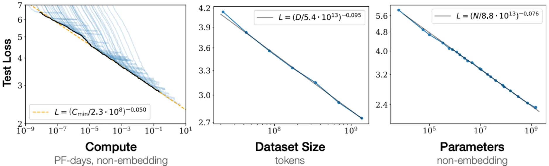
Scaling Laws: Are Transformers All We Need?
Before diving into the technical details, it’s worth understanding why Transformers have become so dominant in NLP.
- With Transformers, language modeling performance improves smoothly as we increase model size, training data, and compute resources in tandem.
- This power-law relationship has been observed over multiple orders of magnitude with no sign of slowing!
- If we keep scaling up these models (with no change to the architecture), could they eventually match or exceed human-level performance?
To Conclude:
- They achieve superior performance on key NLP tasks like machine translation
- They’re more efficient to train than previous approaches
- They scale remarkably well with more data and compute
- Their success has extended beyond NLP to areas like protein folding (AlphaFold 2) and computer vision (Vision Transformers)
The Self-Attention Revolution
The key innovation that made these goals achievable was the self-attention mechanism. Unlike RNNs, which maintain a single hidden state that must capture all relevant information, self-attention allows each word to dynamically gather information from all other words in the sequence. This is analogous to how humans read complex text – we often look back and forth between words to understand their relationships and meaning in context.
At its core, attention is a computational mechanism inspired by human cognition that allows models to focus on specific parts of input data while processing it. Think of attention as a “fuzzy lookup table” - whereas traditional lookup tables map each query to exactly one key-value pair, attention mechanisms allow each query to match multiple keys to varying degrees, returning a weighted sum of values based on these matches. By relating different positions within a sequence, attention layers learn powerful contextual representations over sequential data, making them a key component of modern deep learning architectures.
Queries, keys and values
Self-attention operates like a smart information retrieval system. For every input vector , three different representations are created:
: A vector representing the current focus of attention.
- Compared to all of the other preceding inputs (keys) to establish the weights for its own output .
- Network transforms this representation into the representation of the target token (next token).
- During inference, this is typically the current last token and it doesn’t need to be cached.
: A representation of the input that other queries will compare against.
- Used to establish the weights for the output of the j-th vector
- Cached during inference to avoid recomputation.
- Keys: Vectors associated with all other (preceding) tokens in the input, serve as comparison for current query.
: Representation of the actual content that will be aggregated to form the output.
- Weighted by attention scores to produce the final output for each position.
- Also cached during inference for efficiency.
- Values: Vectors associated with all other tokens, which will be used for the weighted sum (original text) to compute the output vector for the current focus of attention.
Interpretation:
- The similarity between the query and key determines the importance of the value.
- If the attention weight for a specific word is high, it means that the model considers that word highly relevant to understanding the current word’s context.
Classical attention has the advantage that a token can “look” at all previous tokens simultaneously. However, it can be computationally expensive for very long sequences. There are two branches to optimize it, which we will discuss
Soft vs. Hard Attention
Attention as we have described it so far is soft in the sense that a token doesn’t attend to just a single token (or small subset of tokens) but all tokens as a weighted average. This has the advantage of being differentiable and allowing for gradients to flow through the attention mechanism, but also sacrifices efficiency. Hard attention, on the other hand, would involve sampling a single token (or more likely, a specific chunk) to attend to, which is non-differentiable. This is more computationally efficient but harder to train. The main difference is whether or not you are taking a weighted average of tokens or selecting hard chunks.
Global vs. Local Attention
In global attention we take all states to compare and update, while in local attention attends to nearby neighborhoods around the query. Global attention is generally preferred as it can capture long-range dependencies, but local attention can be more efficient and is easier to parallelize.
Recipe for Self-Attention in the Transformer
Step 1: With embeddings stacked in X, calculate queries, keys, and values.
Step 2: Calculate attention scores between query and keys.
Step 3: Take the softmax to normalize attention scores.
Step 4: Take a weighted sum of values.
Final equation:
Making It Work: Key Components
Several crucial elements make transformer decoders effective. Let’s dive into each of these components and understand their role in the attention mechanism.
Scaling the dot product
The scaling factor is a critical yet often overlooked component of the attention mechanism. It was introduced to counteract the effect of having the dot products take on extreme values, as their variance scales with .
Why is this important? Without scaling, as the dimension of the keys () grows, the dot products grow in magnitude, pushing the softmax function into regions where it has extremely small gradients. This leads to vanishing gradients, making the model difficult to train, as well as numerical instability issues.
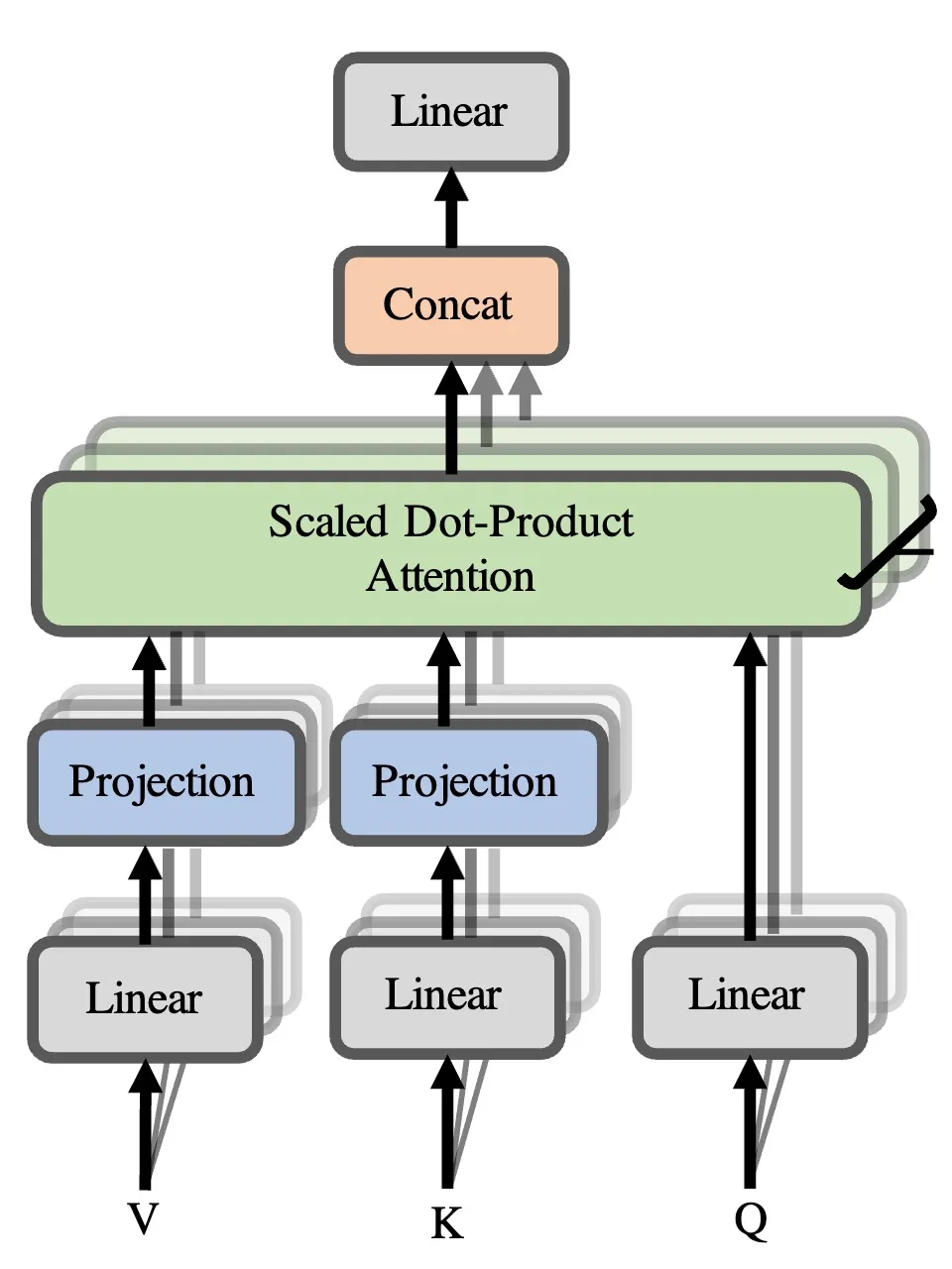
Multi-Head Attention
Rather than having a single attention mechanism, transformers use multiple “heads” of attention in parallel. Each head can learn to focus on different aspects of the input - some might focus on nearby words, others on long-range dependencies, and others on specific linguistic patterns. This allows the model to jointly attend to information from different representation subspaces at different positions.
Benefits of Multi-Head Attention:
- Parallelism: Multiple attention operations can be computed simultaneously.
- Diverse Representations: Each head can learn to focus on different aspects of the input.
- Improved Performance: Empirically, multi-head attention outperforms single-head attention.
Mathematically: In multi-head attention, we can split our entire embedding and pass each part through different matrices — basically, this is multi-head attention, where a head is precisely that split. The results of these independent attention mechanisms are then concatenated and linearly transformed into the required dimension.
For a sneak peek into the multi-head attention code, jump down to Multi-Head Attention (MHA) section below.
Masked Attention
Attention masks are used to control which positions in the input sequence are attended to and which are ignored. Masking is important for handling several scenarios, but perhaps the most important is for autoregressive models, where we want to prevent the model from peeking ahead during training.
Causal language models and causal masking
In causal language models, we want to predict the next word in a sentence. We don’t want to use the information from the future words.This is implemented through “masked” self-attention, where future tokens are hidden during training and inference. This masking is crucial - without it, the model could “cheat” by looking ahead at the answers during training.
At a high-level, we hide (mask) information about future tokens from the model by setting their attention scores to (or a very large negative value) before applying the softmax function. This ensures that the model doesn’t attend to the masked tokens.
Masking the future in self-attention In order to use self-attention in decoders, we need to ensure we can’t peek at the future. To do this we could:
- At every timestep, we could change the set of keys and queries to include only past words. (Inefficient!)
- To enable parallelization, we mask out attention to future words by setting attention scores to .
Attn Scores:   Mask:              Masked Scores:
[[1, 2, 3],    [[0, -inf, -inf],   [[1, -inf, -inf],
 [4, 5, 6],  +  [0,    0, -inf],  = [4,    5, -inf],
 [7, 8, 9]]     [0,    0,    0]]    [7,    8,    9]]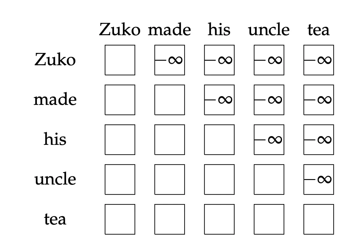
Implementing this masking in code is straightforward. Here’s a simple example in PyTorch:
def masked_attention(query, key, value):
    d_k = query.size(-1)
    scores = torch.matmul(query, key.transpose(-2, -1)) / math.sqrt(d_k)

    # Create mask
    mask = torch.triu(torch.ones_like(scores), diagonal=1).bool()
    scores = scores.masked_fill(mask, float('-inf'))

    attention_weights = torch.softmax(scores, dim=-1)
    return torch.matmul(attention_weights, value)
Padding and Batching
While causal masking prevents the model from attending to future tokens, we also need to consider another type of masking when working with batched inputs of varying lengths: padding masks.
Why Padding is Necessary: In real-world scenarios, sequences in a batch often have different lengths. To process them efficiently in parallel, we pad shorter sequences to match the length of the longest sequence in the batch. However, we don’t want the model to attend to or be influenced by these padding tokens.
Padding Masks: A padding mask is a binary tensor that marks which elements in the input are real tokens (1) and which are padding (0). This mask is used in conjunction with the causal mask to ensure the model only attends to valid, non-future tokens.
Positional Representation
Since attention has no inherent notion of word order, we need to explicitly represent position information. Since attention has no inherent notion of word order, we need to explicitly represent position information. There are two main approaches to incorporate positional information: position embeddings and positional encodings.
Position Embeddings
Position embeddings are learned vectors that are added to the input embeddings to represent the position of each token in the sequence.
In particular, we initialize another parameter matrix , where is the maximum sequence length and is the dimension of the embeddings. The position embedding for the -th token is then given by .
We simply add embedded representation of the position of a token to its token embedding:
and perform self-attention as we otherwise would. Now, the self attention operation can use the embedding to look at the word at position differently than if that word were at position .
The implementation really is just this simple:
class PositionEmbedding(nn.Module):
    def __init__(self, d_model, max_len=5000):
        super().__init__()
        self.embedding = nn.Embedding(max_len, d_model)

    def forward(self, x):
        positions = torch.arange(x.size(1), device=x.device).unsqueeze(0)
        return x + self.embedding(positions)
The drawback is that we have to see sequences of every length during training, otherwise the relevant position embeddings don’t get trained. The benefit is that it works pretty well, and it’s easy to implement.
Positional Encodings
Position encodings work in the same way as embeddings, except that we don’t learn the position vectors, we just choose some function to map the positions to real valued vectors, and let the network figure out how to interpret these encodings. The benefit is that for a well chosen function, the network should be able to deal with sequences that are longer than those it’s seen during training (it’s unlikely to perform well on them, but at least we can check). The drawbacks are that the choice of encoding function is a complicated hyperparameter, and it complicates the implementation a little.
There are a whole host of choices for both embeddings and encodings, which I will cover in a future post. Just to hint at what’s possible, here are a few:
Sinusoidal position encodings:
Concatenate sinusoidal functions of varying periods
and
Pytorch Implementation In order to understand the most common implementation of sinusoidal position encodings, let’s first simplify the denominator. Setting , the denominator is
Thus, we have:
def positional_encoding(seq_len: int, d_model: int, n: float = 10_000.0):
    """Generate positional encodings

    PE(pos, 2i)     = sin(pos/n^(2i/d))
    PE(pos, 2i + 1) = cos(pos/n^(2i/d))

    Args:
        seq_len: int, length of the sequence
        d_model: int, dimension of the model
        n: float, constant set to 10,000

    Returns:
        pos_encoding: torch.Tensor of shape (1, seq_len, d_model)
    """
    position = torch.arange(seq_len).unsqueeze(1).float()
    div_term = torch.exp(torch.arange(0, d_model, 2).float() * -(math.log(n) / d_model))
    pos_encoding = torch.zeros(1, seq_len, d_model)
    pos_encoding[0, :, 0::2] = torch.sin(position * div_term)
    pos_encoding[0, :, 1::2] = torch.cos(position * div_term)
    return pos_encoding
Attention with Linear Bias (ALiBi): attention should look at words “nearby” more than “far” words
where is the key sequence, is the query for the -th token, and is a linear bias term added to make the attention focus more on nearby words.
Feed-Forward Networks (MLPs)
• Problem: Since there are no element-wise non-linearities, self- attention is simply performing a re-averaging of the value vectors. • Easy fix: Apply a feedforward layer to the output of attention, providing non-linear activation (and additional expressive power). After the attention layer, each position goes through a feed-forward neural network. This allows the model to transform the attended information and inject non-linearity into the process.
A modern MLP implementation used in the LLaMA model is not much more complicated than this:
class MLP(nn.Module):
    def __init__(self, dim: int, hidden_dim: int, dropout: float = 0.1):
        super().__init__()
        self.w1 = nn.Linear(dim, hidden_dim)
        self.w2 = nn.Linear(hidden_dim, dim)
        self.w3 = nn.Linear(dim, hidden_dim)
        self.dropout = nn.Dropout(dropout)

    def forward(self, x: torch.Tensor) -> torch.Tensor:
        x = F.silu(self.w1(x)) * self.w3(x)
        x = self.w2(x)
        x = self.dropout(x)
        return x
Training Tricks:
Training Trick #1: Residual Connections [**He et al., 2016]
Residual connections are a simple but powerful technique from computer vision that help in training deep networks by allowing gradients to flow more easily through the network. Deep networks are surprisingly bad at learning the identity function! Therefore, directly passing “raw” embeddings to the next layer can actually be very helpful! This prevents the network from “forgetting” or distorting important information as it is processed by many layers.
class TransformerBlock(nn.Module):
    ...
    def forward(
        self,
        x: torch.Tensor,
    ) -> torch.Tensor:
        """
        norm -> attn -> norm -> mlp
        """
        h = x + self.attn(self.norm1(x))
        h = h + self.mlp(self.norm2(h))
        return h
Training Trick #2: Layer Normalization [Ba et al., 2016]
Problem: It is difficult to train the parameters of a given layer because its input from the layer beneath keeps shifting.
Solution: Reduce variation by normalizing to zero mean and standard deviation of one within each layer.
Two modern normalization techniques are LayerNorm and RMSNorm. Here are simple implementations:
class LayerNorm(nn.Module):
    def __init__(self, dim: int, eps: float = 1e-8):
        super().__init__()
        self.eps = eps
        self.weight = nn.Parameter(torch.ones(dim))
        self.bias = nn.Parameter(torch.zeros(dim))

    def forward(self, x: torch.Tensor) -> torch.Tensor:
        """
        y = (x - mean(x)) / std(x) * weight + bias
        """
        mean = x.mean(dim=-1, keepdim=True)
        std = x.std(dim=-1, keepdim=True)
        x = (x - mean) / (std + self.eps)
        return x * self.weight + self.bias
class RMSNorm(nn.Module):
def __init__(self, dim: int, eps: float = 1e-8):
super().__init__()
self.eps = eps
self.weight = nn.Parameter(torch.ones(dim))
def _norm(self, x: torch.Tensor) -> torch.Tensor:
return x * torch.rsqrt((x ** 2).mean(dim=-1, keepdim=True) + self.eps)
def forward(self, x: torch.Tensor) -> torch.Tensor:
"""
y = x / sqrt(mean(x^2)) * weight
"""
return self._norm(x.float(*)).type_as(x) * self.weightThese components and techniques work together to make transformer models powerful and trainable. In the next section, we’ll discuss some inference tricks that can make transformer models more efficient during deployment.
Inference Tricks
While transformer models are powerful, they can be computationally expensive, especially during inference. Here are some key techniques to optimize inference performance:
KV Caching
KV (Key-Value) caching is one of the most important optimizations for autoregressive decoding in transformers.
How it works:
- Store the key and value tensors for each layer after they’re computed.
- In subsequent steps, only compute the query for the new token and reuse the cached keys and values.
Benefits:
- Significantly reduces computation for long sequences.
- Particularly effective for autoregressive generation.
class KVCache(nn.Module):
    def __init__(
        self,
        max_batch_size: int,
        max_seq_len: int,
        num_heads: int,
        head_dim: int,
        dtype: torch.dtype = torch.float16,
    ):
        super().__init__()
        self.max_batch_size = max_batch_size
        self.max_seq_len = max_seq_len
        self.num_heads = num_heads
        self.head_dim = head_dim
        self.dtype = dtype

        self.init_cache()

    def init_cache(self):
        k_cache = torch.empty(
            self.max_batch_size,
            self.max_seq_len,
            self.num_heads,
            self.head_dim,
            dtype=self.dtype,
        )
        self.register_buffer("k_cache", k_cache)

        v_cache = torch.empty(
            self.max_batch_size,
            self.max_seq_len,
            self.num_heads,
            self.head_dim,
            dtype=self.dtype,
        )
        self.register_buffer("v_cache", v_cache)

class Attention(nn.Module):
    def __init__(self, args):
        super().__init__()
        ...
        self.cache = (
            KVCache(
                args.max_batch_size,
                args.max_seq_len,
                self.n_local_kv_heads,
                self.head_dim,
            )
            if args.max_batch_size > 0
            else None
        )


    def forward(self, x):
        bsz, seqlen, dim = x.size()

        # QKV
        xq, xk, xv = self.wq(x), self.wk(x), self.wv(x)
        xq = xq.view(bsz, seqlen, self.n_local_heads, self.head_dim)
        xk = xk.view(bsz, seqlen, self.n_local_kv_heads, self.head_dim)
        xv = xv.view(bsz, seqlen, self.n_local_kv_heads, self.head_dim)

        # RoPE relative positional embeddings
        xq, xk = apply_rotary_emb(xq, xk, freqs_cos, freqs_sin)

        if self.cache is not None:
            # Update the cache at the provided positions
            scatter_pos = positions[None, :, None, None].repeat(
                bsz, 1, self.n_kv_heads, self.head_dim
            )  # [bsz, positions.shape[0], n_kv_heads, head_dim]
            self.cache.k_cache.scatter_(dim=1, index=scatter_pos, src=xk)
            self.cache.v_cache.scatter_(dim=1, index=scatter_pos, src=xv)

            # grouped multiquery attention: expand out keys and values
            if positions.shape[0] > 1:
                # prefill
                xk, xv = repeat_kv(
                    xk, xv, self.n_rep
                )  # (bs, seqlen, n_local_heads, head_dim)
            else:
                # Retrieve from cache
                cur_pos = positions[-1].item() + 1
                xk, xv = repeat_kv(
                    self.cache.k_cache[:bsz, :cur_pos, ...],
                    self.cache.v_cache[:bsz, :cur_pos, ...],
                    self.n_rep,
                )
        else:
            xk, xv = repeat_kv(xk, xv, self.n_rep)

        # (attn continued)
Beam Search
Beam search is a heuristic search algorithm that explores a graph by expanding the most promising node in a limited set.
How it works:
- Maintain a set of partial hypotheses (the beam).
- At each step, expand each hypothesis in the beam.
- Keep only the top-k expanded hypotheses.
Benefits:
- Often produces better results than greedy decoding.
- Allows exploration of multiple promising paths.
def beam_search(model, start_token, beam_size=4, max_length=50):
    beams = [(start_token, 0)]  # Initialize with start token and score 0
    for _ in range(max_length):
        new_beams = []
        for seq, score in beams:
            logits = model(seq)  # Get predictions for the current sequence
            # Get top k most likely next tokens and their probabilities
            top_k = torch.topk(logits[-1], beam_size)
            for token, prob in zip(top_k.indices, top_k.values):
                # Create new sequences by appending each top-k token
                # Update score by adding log probability of the new token
                new_beams.append((torch.cat([seq, token.unsqueeze(0)]), score + prob.item()))
        # Sort new beams by score (highest first) and keep only the top 'beam_size' beams
        beams = sorted(new_beams, key=lambda x: x[1], reverse=True)[:beam_size]
    return beams[0][0]  # Return the sequence with the highest final score
Key points:
- We maintain a list of
beams, each containing a sequence and its score. - For each step, we expand all current beams by considering the top-k most likely next tokens.
- We sort the new beams by their updated scores and keep only the top
beam_sizebeams. - This process allows us to explore multiple promising paths simultaneously.
Top-k and Top-p (Nucleus) Sampling
These sampling methods provide a balance between diversity and quality in generated text.
Top-k sampling:
- Sample from the k most likely next tokens.
Top-p (nucleus) sampling:
- Sample from the smallest set of tokens whose cumulative probability exceeds p.
def top_k(logits: torch.Tensor, k: int = 0) -> torch.Tensor:
    """Keep only the top k logits."""
    if k == 0:
        return logits
    values, indices = torch.topk(logits, k)
    output = torch.full_like(logits, -math.inf)
    output.scatter_(dim=-1, index=indices, src=values)
    return output

def top_p(logits: torch.Tensor, p: float = 1.0) -> torch.Tensor:
    """Keep smallest set of tokens whose cumulative probability exceeds p."""
    if p == 1.0:
        return logits

    # 1. Sort the logits in descending order
    # 2. Convert to probs
    # 3. Calculate cumulative probabilities
    sorted_logits, sorted_indices = torch.sort(logits, descending=True)
    cumulative_probs = torch.softmax(sorted_logits, dim=-1).cumsum(dim=-1)

    # Remove logits whose cumulative probability exceeds the threshold p
    sorted_logits[cumulative_probs > p] = -math.inf

    # Reorder the logits to their original indices
    output = torch.full_like(logits, -math.inf)
    output.scatter_(dim=-1, index=sorted_indices, src=sorted_logits)
    return output

def sample_top_p(probs: torch.Tensor, p: float = 0.8) -> torch.Tensor:
    return torch.multinomial(probs, num_samples=1)

def sample(
    logits: torch.Tensor,
    temperature: float = 0.0,
    top_p: float = 0.8,
) -> torch.Tensor:
    if temperature > 0:
        probs = torch.softmax(logits / temperature, dim=-1)
        next_token = sample_top_p(probs, top_p)
    else:
        next_token = torch.argmax(logits, dim=-1)[None]

    return next_token.reshape(-1)
Key points:
- Temperature scaling adjusts the “sharpness” of the distribution.
- For top-k, we keep only the k highest probability tokens and set the rest to negative infinity.
- For top-p:
- We sort the logits and calculate cumulative probabilities.
- We find the minimal set of tokens whose cumulative probability exceeds p.
- We remove all tokens outside this set by setting their logits to negative infinity.
- These methods help balance between diversity and quality in generated text.
Quantization
Quantization reduces the precision of the model weights and activations, typically from 32-bit floating point to 8-bit integers.
Benefits:
- Reduces memory usage and computational requirements.
- Can significantly speed up inference, especially on specialized hardware.
def quantize_tensor(x, num_bits=8):
    qmin, qmax = 0, 2**num_bits - 1  # Define the range of quantized values
    min_val, max_val = x.min(), x.max()  # Find the range of the input tensor
    # Calculate the scale and zero point for quantization
    scale = (max_val - min_val) / (qmax - qmin)
    zero_point = qmin - min_val / scale
    # Quantize the tensor
    q_x = torch.round(x / scale + zero_point)
    q_x = torch.clamp(q_x, qmin, qmax).byte()  # Ensure values are within range and convert to bytes
    return q_x, scale, zero_point

def dequantize_tensor(q_x, scale, zero_point):
    # Convert quantized values back to original scale
    return scale * (q_x.float() - zero_point)
Key points:
- Quantization maps floating-point values to a fixed set of integers (usually 256 values for 8-bit quantization).
- We calculate a
scaleandzero_pointto map the full range of the input to the quantized range. - The quantization formula is: q = round(x / scale + zero_point)
- Dequantization reverses this process: x = scale * (q - zero_point)
- This process significantly reduces memory usage and can speed up computations, especially on specialized hardware.
Attention and all its variants
We’ll cover the following:
- Attention: The basic attention module
- Multi-head Attention: A multi-head attention module that performs attention on multiple different “heads”(each head is a set of Q, K, V) of the input sequence.
- Multi-Query Attention: A multi-query attention module that allows multiple queries and only one key, value to attend to the same input sequence.
- Grouped-Query Attention: A grouped query attention module that allows queries to be grouped together (each group include multiple queries and only one key) and attended to jointly.
- Linformer: which reduces the overall self-attention complexity from O(n2) to O(n) in both time and space.
Single-Head Attention (SA)
Single-head attention is the simplest form of attention mechanism. It computes the attention scores between a query and a set of key-value pairs. The attention score is computed as the dot product between the query and the keys, followed by a softmax operation. The output is the weighted sum of the values, where the weights are the attention scores.
class SingleHeadAttention(nn.Module):
    """Single head attention mechanism.

    For learning purposes, we will implement the single head attention mechanism.
    """

    def __init__(
        self,
        dim: int,
        head_dim: int,
        dropout: float = 0.1,
        max_seq_len: int = 32768,
    ):
        super().__init__()
        self.dim = dim
        self.head_dim = head_dim
        self.wq = nn.Linear(dim, head_dim)
        self.wk = nn.Linear(dim, head_dim)
        self.wv = nn.Linear(dim, head_dim)
        self.wo = nn.Linear(head_dim, dim)
        self.attn_dropout = nn.Dropout(dropout)
        self.resid_dropout = nn.Dropout(dropout)
        self.max_seq_len = max_seq_len
        mask = torch.full((1, self.max_seq_len, self.max_seq_len), float("-inf"))
        mask = torch.triu(mask, diagonal=1)
        self.register_buffer("mask", mask)

    def forward(self, x: torch.Tensor) -> torch.Tensor:
        """Forward pass of the single head attention mechanism.

        Args:
            x (torch.Tensor): The input tensor.

        Returns:
            torch.Tensor: The output tensor.
        """
        k, q, v = self.wk(x), self.wq(x), self.wv(x)

        # Scaled dot product attention
        scores = torch.matmul(q, k.transpose(-2, -1)) / self.head_dim**0.5
        # Mask out the upper triangular part of the matrix
        scores = scores + self.mask[:, : scores.size(1), : scores.size(2)]

        attn = F.softmax(scores, dim=-1)
        attn = self.attn_dropout(attn)
        output = torch.matmul(attn, v)
        output = self.wo(output)
        output = self.resid_dropout(output)
        return output
Multi-Head Attention (MHA)
Multi-head attention extends single-head attention by computing multiple attention scores in parallel. Each head has its own set of learnable parameters, and the outputs are concatenated and linearly transformed to produce the final output.
Multi-head attention has query, key, and value heads.
class MultiHeadAttention(nn.Module):

    def __init__(
        self,
        dim: int,
        num_heads: int,
        num_kv_heads: Optional[int] = None,
        dropout: float = 0.1,
        max_seq_len: int = 32768,
    ):
        super().__init__()
        self.dim = dim
        self.num_heads_q = num_heads
        self.head_dim = dim // num_heads
        self.max_seq_len = max_seq_len

        self.num_heads_kv = num_kv_heads if num_kv_heads is not None else num_heads
        self.num_rep = self.num_heads_q // self.num_heads_kv

        self.attn_dropout = nn.Dropout(dropout)
        self.resid_dropout = nn.Dropout(dropout)
        self.wq = nn.Linear(dim, self.num_heads_q * self.head_dim, bias=False)
        self.wk = nn.Linear(dim, self.num_heads_kv * self.head_dim, bias=False)
        self.wv = nn.Linear(dim, self.num_heads_kv * self.head_dim, bias=False)
        self.wo = nn.Linear(self.num_heads_q * self.head_dim, dim, bias=False)

        mask = torch.full((1, 1, max_seq_len, max_seq_len), float("-inf"))
        self.register_buffer("mask", torch.triu(mask, diagonal=1))

    def forward(self, x: torch.Tensor) -> torch.Tensor:
        """Forward pass of the single head attention mechanism.

        Args:
            x (torch.Tensor): The input tensor.

        Returns:
            torch.Tensor: The output tensor.
        """

        k, q, v = self.wk(x), self.wq(x), self.wv(x)

        # Reshape the tensors to have the same number of heads
        xq: torch.Tensor = xq.view(bsz, seqlen, self.num_heads_q, self.head_dim)
        xk: torch.Tensor = xk.view(bsz, seqlen, self.num_heads_kv, self.head_dim)
        xv: torch.Tensor = xv.view(bsz, seqlen, self.num_heads_kv, self.head_dim)

        # move heads into batch dimension
        xq = xq.transpose(1, 2)  # [bs, num_heads, seqlen, head_dim]
        xk = xk.transpose(1, 2)  # [bs, num_heads, seqlen, head_dim]
        xv = xv.transpose(1, 2)  # [bs, num_heads, seqlen, head_dim]

        # Scaled dot product attention
        scores = torch.matmul(xq, xk.transpose(2, 3)) / math.sqrt(self.head_dim)
        scores = scores + self.mask[:, :, :seqlen, :seqlen]
        scores = F.softmax(scores, dim=-1).type_as(xq)
        scores = self.attn_dropout(scores)
        output = torch.matmul(scores, xv)  # [bs, num_heads, seqlen, head_dim]

        # restore seqlen into batch dim and concatenate heado
        output = output.transpose(1, 2).contiguous().view(bsz, seqlen, -1)

        # Project to the output dimension + residual
        output = self.wo(output)
        output = self.resid_dropout(output)
        return output
Multi-Query Attention (MQA)
Multi-query attention [1] is the same as multi-head attention, except it uses a single shared key-value head (i.e., the different heads share a single set of keys, values and outputs). The queries are not shared across heads.
Multi-query attention shares single key and value heads across all query heads.
MQA drastically speeds up decoder inference.
class MultiQueryAttention(nn.Module):
    r"""
    https://arxiv.org/pdf/1911.02150.pdf

    Uses only a single key-value head
    - drastically speeds up decoder inference, but can lead to quality degredation.

    Exactly the same as multi-head attention except that the different heads
    share the same keys and values (but queries are not shared).
    """

    def __init__(
        self,
        dim: int = 512,
        head_dim: int = 64,
        num_heads_q: int = 8,
        max_seq_len: int = 32768,
    ) -> None:
        self.dim = dim
        self.num_heads_q = num_heads_q
        self.head_dim = head_dim
        self.max_seq_len = max_seq_len

        self.wq = nn.Linear(dim, self.num_heads_q * head_dim, bias=False)
        self.wk = nn.Linear(dim, head_dim, bias=False)
        self.wv = nn.Linear(dim, head_dim, bias=False)
        self.wo = nn.Linear(self.num_heads_q * head_dim, dim, bias=False)
        mask = torch.full((1, 1, max_seq_len, max_seq_len), float("-inf"))
        self.register_buffer("mask", torch.triu(mask, diagonal=1))

    def forward(self, x: Tensor):
        bsz, seq_len, dim = x.size()

        # Below, we see that queries (xq) are split into num_heads_q parts
        xq = self.wq(x).view(bsz, seq_len, self.num_heads_q, self.head_dim)
        xk = self.wk(x)
        xv = self.wv(x)

        # Einsum first broadcasts xk to have the same shape as xq
        # xk -> (bsz, seq_len, 1, head_dim)
        # Then, to compute the dot product, the singleton dimension is repeated to match the number of heads, and the dot product is computed over the last dimension
        # Finally, we can see that the output shape calls for moving the num_heads_q dimension to the second dimension
        scores = torch.einsum("bshd, bnd -> bhsn", xq, xk) / math.sqrt(dim)

        weights = torch.softmax(scores, dim=-1)
        out = torch.einsum("bhsn, bnd -> bhnd", weights, xv)
        out = out.transpose(1, 2).contiguous().view(bsz, seq_len, -1)
        return self.wo(out)
Grouped-Query Attention (GQA)
Grouped-query [2] attention is a generalization of multi-query attention which uses an intermediate (more than one, less than number of query heads) number of key-value heads. GQA addresses the issue of quality degradation of MQA. GQA is a trade-off between MQA and MHA, and comes with a recipe that allows for up-training existing MHA checkpoints into models with MQA or GQA.
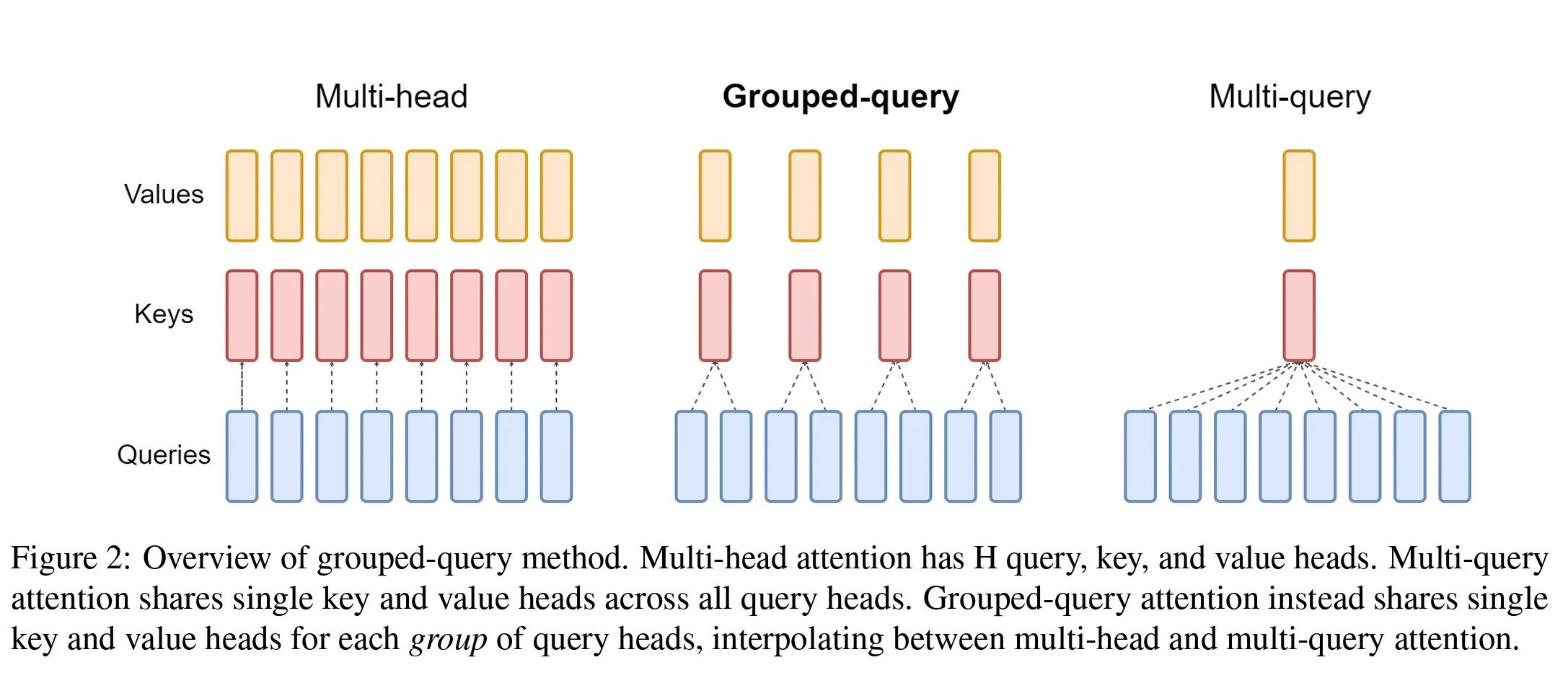
Grouped-query attention instead shares single key and value heads for each group of query heads, interpolating between multi-head and multi-query attention.
GQA divides query heads into groups (GQA), each of which shares a single key head and value head. GQA is equivalent to MQA, and GQA is equivalent to MHA.
class GroupedQueryAttention(nn.Module):
r"""
https://arxiv.org/pdf/2305.13245.pdf
GQA divides query heads into $G$ groups (GQA$-G$),
each of which shares a single key head and value head.
GQA$-1$ is equivalent to MQA, and GQA$-H$ is equivalent to MHA.
"""
def __init__(
self,
dim: int = 512,
head_dim: int = 64,
num_heads_q: int = 8,
num_heads_kv: int | None = None,
max_seq_len: int = 32768,
) -> None:
super().__init__()
self.dim = dim
self.head_dim = head_dim
self.num_heads_q = num_heads_q
self.num_heads_kv = num_heads_kv if num_heads_kv is not None else num_heads_q
self.num_rep = self.num_heads_q // self.num_heads_kv
self.max_seq_len = max_seq_len
self.wq = nn.Linear(dim, self.num_heads_q * head_dim, bias=False)
self.wk = nn.Linear(dim, self.num_heads_kv * head_dim, bias=False)
self.wv = nn.Linear(dim, self.num_heads_kv * head_dim, bias=False)
self.wo = nn.Linear(self.num_heads_q * head_dim, dim, bias=False)
mask = torch.full((1, 1, max_seq_len, max_seq_len), float("-inf"))
self.register_buffer("mask", torch.triu(mask, diagonal=1))
def forward(self, x: Tensor):
bsz, seq_len, dim = x.size()
xq = self.wq(x).view(bsz, seq_len, self.num_heads_q, self.head_dim)
xk = self.wk(x).view(bsz, seq_len, self.num_heads_kv, self.head_dim)
xv = self.wv(x).view(bsz, seq_len, self.num_heads_kv, self.head_dim)
xq = xq.transpose(1, 2).view(
bsz, self.num_rep, self.num_heads_kv, seq_len, self.head_dim
)
xk = xk.transpose(1, 2) # [b x h x n x d]
xv = xv.transpose(1, 2) # [b x h x n x d]
# xk and xv get repeated due to broadcasting
scores = torch.einsum("bghnd, bhsd -> bghns", xq, xk) / math.sqrt(dim)
weights = torch.softmax(scores, dim=-1)
out = torch.einsum("bghns, bhnd -> bghnd", weights, xv)
out = out.permute(0, 3, 1, 2, 4).reshape(bsz, seq_len, -1).contiguous()
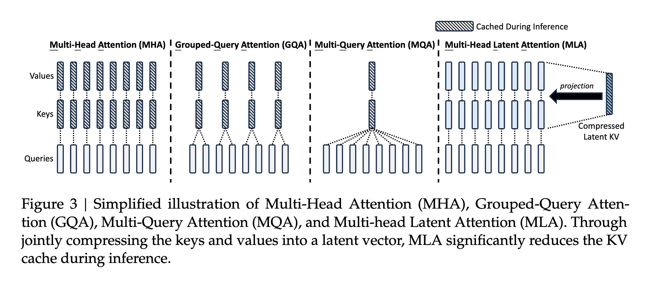
return self.wo(out)Multi-head Latent Attention (MLA)
Multi-head Latent Attention (MLA) was first introduced in DeepSeek-V2 [3] attempting to provide further computational gains by compressing KV layers/cache into latent states using low-rank matrices. Instead of reducing the number of KV-heads, MLA compresses the keys and values into a latent space, reducing the number of parameters and computational complexity.
Low-rank Key-Value Joint Compression
The mechanism for low-rank joint compression for keys and values to reduce the KV cache uses the following:
where:
- is the latent vector for keys and values
- () denotes the KV compression dimension
- is the down-projection matrix
- are the up-projection matrices for keys.
During training, compression for the queries can also be performed to reduce activation memory.
Decoupled Rotary Position Embedding
Standard Rotary Position Embedding (RoPE) is incompatible with low-rank KV compression because RoPE is position-sensitive for both keys and queries. The solution is to use additional multi-head queries and a shared key for the RoPE, which allows for decoupling of the RoPE from the main attention mechanism.
where and are matrices to produce3 the decoupled queries and key.
Comparison of Key-Value Cache
| Attention Mechanism | KV Cache per Token (# Element) | Capability |
|---|---|---|
| Multi-Head Attention (MHA) | Strong | |
| Grouped-Query Attention (GQA) | Moderate | |
| Multi-Query Attention (MQA) | Weak | |
| Multi-head Latent Attn (MLA) | Stronger |
Table | Comparison of the KV cache per token among different attention mechanisms.
- denotes the number of attention heads
- denotes the dimension per attention head
- denotes the number of layers
- denotes the number of groups in GQA
- and denote the KV compression dimension and the per-head dimension of the decoupled queries and key in MLA, respectively.
import math
import torch
import torch.nn as nn
import torch.nn.functional as F
def precompute_freqs_cis(dim: int, end: int, theta: float = 10000.0):
numerator = torch.arange(0, dim, 2, dtype=torch.float)[: (dim // 2)] / dim
freqs = 1 / (theta**numerator)
t = torch.arange(end, device=freqs.device, dtype=freqs.dtype)
freqs = torch.outer(t, freqs).float()
return torch.polar(torch.ones_like(freqs), freqs)
def reshape_for_broadcast(freqs_cis: torch.Tensor, x: torch.Tensor):
ndim = x.ndim
assert 0 <= 1 < ndim
assert freqs_cis.shape == (x.shape[1], x.shape[-1])
shape = [d if i == 1 or i == ndim - 1 else 1 for i, d in enumerate(x.shape)]
return freqs_cis.view(*shape)
def apply_rotary_emb(
xq: torch.Tensor,
xk: torch.Tensor,
freqs_cis: torch.Tensor,
) -> tuple[torch.Tensor, torch.Tensor]:
# Validate input dimensions
assert (
xq.shape[-1] == xk.shape[-1]
), "Query and Key must have same embedding dimension"
assert xq.shape[-1] % 2 == 0, "Embedding dimension must be even"
# Get sequence lengths
q_len = xq.shape[1]
k_len = xk.shape[1]
# Use appropriate part of freqs_cis for each sequence
q_freqs = freqs_cis[:q_len]
k_freqs = freqs_cis[:k_len]
# Apply rotary embeddings separately
# split last dimention to [xq.shape[:-1]/2, 2]
xq_ = torch.view_as_complex(xq.float().reshape(*xq.shape[:-1], -1, 2))
xk_ = torch.view_as_complex(xk.float().reshape(*xk.shape[:-1], -1, 2))
# Reshape freqs for each
q_freqs = reshape_for_broadcast(q_freqs, xq_)
k_freqs = reshape_for_broadcast(k_freqs, xk_)
# Works for both [bsz, seqlen, n_heads*head_dim] and [bsz, seqlen, n_heads, head_dim]
xq_out = torch.view_as_real(xq_ * q_freqs).flatten(xq.ndim - 1)
xk_out = torch.view_as_real(xk_ * k_freqs).flatten(xk.ndim - 1)
return xq_out.type_as(xq), xk_out.type_as(xk)
class MultiHeadLatentAttention(nn.Module):
def __init__(
self,
dim: int = 512,
head_dim: int = 64,
num_heads: int = 8,
dc_kv: int = 64,
dc_q: int = 64,
d_rope: int = 32,
dropout=0.0,
max_seq_len=8129,
bias: bool = False,
max_batch_size: int = 32,
):
super().__init__()
self.dim = dim
self.head_dim = head_dim
self.max_seq_len = max_seq_len
self.num_heads = num_heads
self.d_rope = d_rope
# Linear down-projections (compressions)
self.w_dq = nn.Linear(dim, dc_q, bias=bias)
self.w_dkv = nn.Linear(dim, dc_kv, bias=bias)
# Linear up-projections
self.w_uq = nn.Linear(dc_q, num_heads * head_dim, bias=bias)
self.w_uk = nn.Linear(dc_kv, num_heads * head_dim, bias=bias)
self.w_uv = nn.Linear(dc_kv, num_heads * head_dim, bias=bias)
# Linear RoPE projections
self.w_qr = nn.Linear(dc_q, num_heads * d_rope, bias=bias)
self.w_kr = nn.Linear(dim, d_rope, bias=bias)
self.w_out = nn.Linear(num_heads * head_dim, dim, bias=bias)
self.scale = 1 / math.sqrt(head_dim + d_rope)
self.attn_dropout = torch.nn.Dropout(dropout)
self.res_dropout = torch.nn.Dropout(dropout)
# Initialize freqs_cis for RoPE
self.freqs_cis = precompute_freqs_cis(d_rope, max_seq_len * 2)
# Initialize C_KV and R_K cache for inference
self.cache_kv = torch.zeros((max_batch_size, max_seq_len, dc_kv))
self.cache_kr = torch.zeros((max_batch_size, max_seq_len, d_rope))
def forward(
self,
x: torch.Tensor,
key_value_states=None,
mask: torch.Tensor | None = None,
use_cache: bool = False,
start_pos: int = 0,
):
"""
Forward pass supporting both standard attention and cached inference
Input shape: [bsz, seq_len, dim=num_heads * head_dim]
Args:
sequence: Input sequence [bsz, seq_len, dim]
key_value_states: Optional states for cross-attention
att_mask: Optional attention mask
use_cache: Whether to use KV caching (for inference)
start_pos: Position in sequence when using KV cache
"""
bsz, seq_len, dim = x.shape
self.freqs_cis = self.freqs_cis.to(x.device)
freqs_cis = self.freqs_cis[start_pos:]
# if key_value_states are provided this layer is used as a cross-attention layer
# for the decoder
is_cross_attention = key_value_states is not None
# Determine kv_seq_len early
kv_seq_len = key_value_states.size(1) if is_cross_attention else seq_len
c_q = self.w_dq(x) # [bsz, seq_len, dc_q]
x_q = self.w_uq(c_q).view(bsz, seq_len, self.num_heads, self.head_dim)
x_qr = self.w_qr(c_q).view(bsz, seq_len, self.num_heads, self.d_rope)
kv_inputs = key_value_states if is_cross_attention else x
if use_cache:
# Equation (41) in DeepSeek-v2 paper: cache c^{KV}_t
self.cache_kv = self.cache_kv.to(x.device)
# Get current compressed KV states
current_kv = self.w_dkv(kv_inputs) # [batch_size, kv_seq_len, d_c]
# Update cache using kv_seq_len instead of seq_len
self.cache_kv[:bsz, start_pos : start_pos + kv_seq_len] = current_kv
# Use cached compressed KV up to current position
c_kv = self.cache_kv[:bsz, : start_pos + kv_seq_len]
# Equation (43) in DeepSeek-v2 paper: cache the RoPE pathwway for shared key k^R_t
assert (
self.cache_kr.size(-1) == self.d_rope
), "RoPE cache dimension mismatch"
self.cache_kr = self.cache_kr.to(x.device)
# Get current RoPE key
current_x_kr = self.w_kr(kv_inputs) # [bsz, seq_len, d_rope]
# Update cache using kv_seq_len instead of seq_len
self.cache_kr[:bsz, start_pos : start_pos + seq_len] = current_x_kr
# Use cached RoPE key up to current position
x_kr = self.cache_kr[
:bsz, : start_pos + kv_seq_len
] # [bsz, cached_len, d_rope]
"""handling attention mask"""
if mask is not None:
# Get the original mask shape
cached_len = (
start_pos + kv_seq_len
) # cached key_len, including previous key
assert (
c_kv.size(1) == cached_len
), f"Cached key/value length {c_kv.size(1)} doesn't match theoretical length {cached_len}"
# Create new mask matching attention matrix shape
extended_mask = torch.zeros(
(
bsz,
1,
seq_len,
cached_len,
), # [batch, head, query_len, key_len]
device=mask.device,
dtype=mask.dtype,
)
# Fill in the mask appropriately - we need to be careful about the causality here
# For each query position, it should only attend to cached positions up to that point
for i in range(seq_len):
extended_mask[:, :, i, : (start_pos + i + 1)] = 0 # Can attend
extended_mask[:, :, i, (start_pos + i + 1) :] = float(
"-inf"
) # Cannot attend
mask = extended_mask
else:
c_kv = self.w_dkv(kv_inputs) # [bsz, seq_len, dc_kv]
x_kr = self.w_kr(kv_inputs)
x_k = self.w_uk(c_kv) # [bsz, seq_len, num_heads * head_dim]
x_v = self.w_uv(c_kv) # [bsz, seq_len, num_heads * head_dim]
# After getting x_k from projection, get its actual sequence length
actual_kv_len = x_k.size(1) # kv_seq_len or start_pos + kv_seq_len
# in cross-attention, key/value sequence length might be different from query sequence length
# Use actual_kv_len instead of kv_seq_len for reshaping
x_k = x_k.view(bsz, actual_kv_len, self.num_heads, self.head_dim)
x_v = x_v.view(bsz, actual_kv_len, self.num_heads, self.head_dim)
# Apply RoPE to query and shared key
x_qr = x_qr.view(bsz, seq_len, self.num_heads, self.d_rope)
x_kr = x_kr.unsqueeze(2).expand(
-1, -1, self.num_heads, -1
) # [batch, cached_len, num_heads, d_rotate]
x_qr, x_kr = apply_rotary_emb(x_qr, x_kr, freqs_cis=freqs_cis)
# Concatenate along head dimension
x_q = torch.cat(
[x_q, x_qr], dim=-1
) # [bsz, seq_len, num_heads, head_dim + d_rope]
x_k = torch.cat(
[x_k, x_kr], dim=-1
) # [bsz, actual_kv_len, num_heads, head_dim + d_rope]
# Scale Q by 1/sqrt(d_k)
x_q = x_q * self.scale
x_q = x_q.transpose(1, 2) # [bsz, num_heads, seq_len, head_dim]
x_k = x_k.transpose(1, 2) # [bsz, num_heads, actual_kv_len, head_dim]
x_v = x_v.transpose(1, 2) # [bsz, num_heads, actual_kv_len, head_dim]
# Compute attention scores
attn = torch.matmul(x_q, x_k.transpose(-2, -1))
# apply attention mask to attention matrix
if mask is not None and not isinstance(mask, torch.Tensor):
raise TypeError("att_mask must be a torch.Tensor")
if mask is not None:
attn = attn + mask
else:
mask = torch.full((1, 1, seq_len, kv_seq_len), float("-inf"), device=x.device)
mask = torch.triu(mask, diagonal=1)
attn = attn + mask
scores = F.softmax(attn, dim=-1)
scores = self.attn_dropout(scores)
attn_out = torch.matmul(scores, x_v)
# concatinate all attention heads
attn_out = (
attn_out.transpose(1, 2)
.contiguous()
.view(bsz, seq_len, self.num_heads * self.head_dim)
)
# final linear transformation to the concatenated output
output = self.w_out(attn_out)
output = self.res_dropout(output)
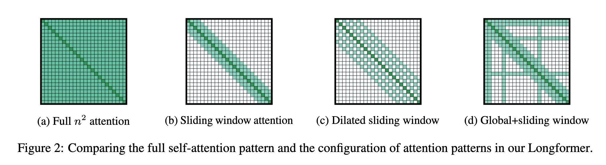
return outputSliding-Window Attention (SWA)
Introduced by Longformer [4] and used in Mistral 7B v0.1 [5], sliding-window attention attempts to alleviate the complexity of the standard self-attention by restricting the attention for a given query to a local window of size . The window is centered around the query, and the attention is computed only for the tokens within the window. So, a token at position in can attend to tokens in the range in . The computational complexity of SWA is ., which scales linearly with the input sequence length and the window size. To make this pattern efficient, should be small compared to . With multiple stacked layers, the overall receptive field can be increased., analogous to CNNs where stacking layers of small kernels leads to high level features that are built from a large portion of the input. In this case, with a transformer of layers, the receptive field size is (assuming is fixed for all layers).
  def chunk(hidden_states: torch.Tensor, window_overlap):
    """convert into overlapping chunks. Chunk size = 2w, overlap = w"""
    bsz, seq_len, dim = hidden_states.size()
    chunk_size = [
        bsz,
        # n_chunks
        torch.div(seq_len, window_overlap, rounding_mode="trunc") - 1,
        2 * window_overlap,
        dim,
    ]
    overlapping_chunks = torch.empty(
        chunk_size, dtype=hidden_states.dtype, device=hidden_states.device
    )
    for i in range(overlapping_chunks.size(1)):
        overlapping_chunks[:, i] = hidden_states[
            :, i * window_overlap : i * window_overlap + 2 * window_overlap
        ]
    return overlapping_chunks
def sliding_window(
x: torch.Tensor,
window_size: int,
step: int | None = None,
seq_dim: int = 1,
):
"""Slide a window of size `window_size` with step `step` over `x` at dimension `seq_dim`.
Args:
x: input tensor
window_size: size of the window
step: step of the sliding window. If None, step is equal to `window_size`
seq_dim: dimension where the sliding window should be applied
Returns:
"""
if step is None:
step = window_size
if step < 1:
raise ValueError("`step` must be a positive integer")
if window_size < 1:
raise ValueError("`window_size` must be a positive integer")
if window_size > x.size(seq_dim):
raise ValueError(
"`window_size` must be less than the size of the sequence dimension"
)
return x.unfold(seq_dim, window_size, step).transpose(seq_dim + 1, -1)Sliding Window Attention Forward
class LongformerSelfAttention(nn.Module):
    ...
    def _sliding_chunks_query_key_matmul(
        self, query: torch.Tensor, key: torch.Tensor, window_overlap: int
    ):
        """
        Matrix multiplication of query and key tensors using with a sliding window attention pattern.
        This implementation splits the input into overlapping chunks of size 2w
        (e.g. 512 for pretrained Longformer) with an overlap of size window_overlap.
        """
        batch_size, seq_len, num_heads, head_dim = query.size()
        assert (
            seq_len % (window_overlap * 2) == 0
        ), f"Sequence length should be multiple of {window_overlap * 2}. Given {seq_len}"
        assert query.size() == key.size()

        chunks_count = int(
            torch.div(seq_len, window_overlap, rounding_mode="trunc") - 1
        )

        # group batch_size and num_heads dimensions into one,
        # then chunk seq_len into chunks of size window_overlap * 2
        query = query.transpose(1, 2).reshape(batch_size * num_heads, seq_len, head_dim)
        key = key.transpose(1, 2).reshape(batch_size * num_heads, seq_len, head_dim)

        query = sliding_window(query, 2 * window_overlap, window_overlap)
        key = sliding_window(key, 2 * window_overlap, window_overlap)

        # matrix multiplication
        # bcxd: batch_size * num_heads x chunks x 2window_overlap x head_dim
        # bcyd: batch_size * num_heads x chunks x 2window_overlap x head_dim
        # bcxy: batch_size * num_heads x chunks x 2window_overlap x 2window_overlap
        diagonal_chunked_attention_scores = torch.einsum(
            "bcxd,bcyd->bcxy", (query, key)
        )  # multiply

        # convert diagonals into columns
        diagonal_chunked_attention_scores = self._pad_and_transpose_last_two_dims(
            diagonal_chunked_attention_scores, padding=(0, 0, 0, 1)
        )

        # allocate space for the overall attention matrix where the chunks are combined.
        # The last dimension has (window_overlap * 2 + 1) columns.
        # The first (window_overlap) columns are the window_overlap lower triangles
        # (attention from a word to window_overlap previous words).
        # The following column is attention score from each word to itself, then
        # followed by window_overlap columns for the upper triangle.

        diagonal_attention_scores = diagonal_chunked_attention_scores.new_zeros(
            (
                batch_size * num_heads,
                chunks_count + 1,
                window_overlap,
                window_overlap * 2 + 1,
            )
        )

        # copy parts from diagonal_chunked_attention_scores into the combined matrix of attentions
        # - copying the main diagonal and the upper triangle
        diagonal_attention_scores[:, :-1, :, window_overlap:] = (
            diagonal_chunked_attention_scores[
                :, :, :window_overlap, : window_overlap + 1
            ]
        )
        diagonal_attention_scores[:, -1, :, window_overlap:] = (
            diagonal_chunked_attention_scores[
                :, -1, window_overlap:, : window_overlap + 1
            ]
        )
        # - copying the lower triangle
        diagonal_attention_scores[:, 1:, :, :window_overlap] = (
            diagonal_chunked_attention_scores[
                :, :, -(window_overlap + 1) : -1, window_overlap + 1 :
            ]
        )

        diagonal_attention_scores[:, 0, 1:window_overlap, 1:window_overlap] = (
            diagonal_chunked_attention_scores[
                :, 0, : window_overlap - 1, 1 - window_overlap :
            ]
        )

        # separate batch_size and num_heads dimensions again
        diagonal_attention_scores = diagonal_attention_scores.view(
            batch_size, num_heads, seq_len, 2 * window_overlap + 1
        ).transpose(2, 1)

        self._mask_invalid_locations(diagonal_attention_scores, window_overlap)
        return diagonal_attention_scores
Linformer
jhe standard self-attention mechanism of the Transformer uses time and space with respect to sequence length. Linformer [6] reduces the overall self-attention complexity from to in both time and space by approximating it with a low-rank matrix.
class LinearSelfAttention(nn.Module):
    r"""
    https://arxiv.org/abs/2006.04768
    """

    def __init__(
        self,
        dim: int,
        head_dim: int,
        dropout: float = 0.1,
        max_seq_len: int = 32768,
        k: int | None = None,
    ):
        super().__init__()
        self.dim = dim
        self.head_dim = head_dim
        self.wq = nn.Linear(dim, head_dim)
        self.wk = nn.Linear(dim, head_dim)
        self.wv = nn.Linear(dim, head_dim)
        self.wo = nn.Linear(head_dim, dim)
        self.attn_dropout = nn.Dropout(dropout)
        self.resid_dropout = nn.Dropout(dropout)
        self.max_seq_len = max_seq_len
        mask = torch.full((1, self.max_seq_len, self.max_seq_len), float("-inf"))
        mask = torch.triu(mask, diagonal=1)
        self.register_buffer("mask", mask)

        if k is None:
            k = n // 4
        self.k = k
        self.proj_E = nn.Linear(in_features=self.max_seq_len, out_features=k, bias=True)
        self.proj_F = nn.Linear(in_features=self.max_seq_len, out_features=k, bias=True)

    def forward(self, x: torch.Tensor) -> torch.Tensor:
        """Forward pass of the single head attention mechanism.

        Args:
            x (torch.Tensor): The input tensor.

        Returns:
            torch.Tensor: The output tensor.
        """
        k, q, v = self.wk(x), self.wq(x), self.wv(x)

        # Handle a smaller dimension than expected
        padding = 0
        if q.shape[1] < self.max_seq_len:
            padding = self.max_seq_len: - q.shape[1]
            pad_dims = (0, 0, 0, padding)
            q = F.pad(q, pad_dims)
            k = F.pad(k, pad_dims)
            v = F.pad(v, pad_dims)

        k_projected = self.proj_E(k.transpose(-2, -1)).transpose(-2, -1)
        v_projected = self.proj_F(v.transpose(-2, -1)).transpose(-2, -1)

        z = F.scaled_dot_product_attention(q, k_projected, v_projected)
        return z[:, :-padding, :] if padding > 0 else z
AttentionFree Transformer (AFT)
Attention Free Transformer [7] is an efficient variant of a multi-head attention module that does away dot product self attention. In an AFT layer, the key and value are first combined with a set of learned position biases, the result of which is multiplied with the query in an element-wise fashion. This new operation has a memory complexity linear w.r.t. both the context size and the dimension of features, making it compatible to both large input and model sizes. The memory complexity is where is the sequence length and is the dimensionality of the input.
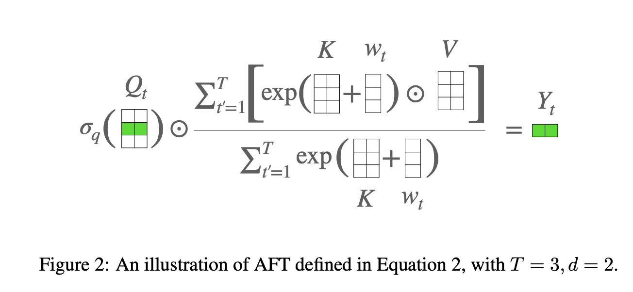
Given an input , AFT first linearly projects it to , , and , as in the standard multi-head attention. The key and value are then combined with a set of learned position biases, and the result is multiplied with the query in an element-wise fashion:
where
- is a learnable pair-wise position biases
- is a non-linear activation function, such as sigmoid.
AFT in Matrix Form
We can write AFT in matrix form by leveraging the rules of exponentiation, allow us replace the exponentiation of the sum with the product of the exponentiations:
So we have
where
- denotes matrix multiplication and denotes element-wise multiplication.
- the matrix multiplication performs the summation over the sequence length , capturing .
In terms of shapes with broadcasting, we have:
W: [1, t, t']
K: [bsz, t', d]
V: [bsz, t', d]
K*V: [bsz, t', d] (element-wise multiplication)
So,
W @ K -> [1, t, t'] @ [bsz, t', d] = [bsz, t, d]
and,
W @ K*V -> [1, t, t'] @ [bsz, t', d] = [bsz, t, d]
Intuitively, for each target position in the input sequence, AFT performs a weighted average of the values, which is combined with the query in an element-wise fashion. The weighting is simply the keys with an added learned pair-wise position bias. Together, this eliminates the need to compute the full attention matrix, making it more memory-efficient.
AFT Full Implementation
import torch
import torch.nn as nn


class AFTFull(nn.Module):
    def __init__(
        self,
        dim: int = 512,
        max_seq_len: int = 2048,
        bias: bool = False,
        w_dim: int = 128,
    ):
        super().__init__()
        self.dim = dim
        self.max_seq_len = max_seq_len

        self.wq = nn.Linear(dim, dim, bias=bias)
        self.wk = nn.Linear(dim, dim, bias=bias)
        self.wv = nn.Linear(dim, dim, bias=bias)
        self.wo = nn.Linear(dim, dim, bias=bias)

        self.activation = nn.Sigmoid()
        self.u = nn.Parameter(torch.randn(1, max_seq_len, w_dim))
        self.v = nn.Parameter(torch.randn(1, max_seq_len, w_dim))
        nn.init.kaiming_uniform_(self.u)
        nn.init.kaiming_uniform_(self.v)
        # wbias = uvT
        # self.wbias = nn.Parameter(torch.randn(1, max_seq_len, max_seq_len))

    def forward(self, x: torch.Tensor):
        """

        Y = sigma(Q) * (W @ K*V) / (W @ K)
        """
        bsz, seqlen, dim = x.shape
        xq: torch.Tensor = self.wq(x)  # [bsz, t', d]
        xk: torch.Tensor = self.wk(x)  # [bsz, t', d]
        xv: torch.Tensor = self.wv(x)  # [bsz, t', d]

        wbias = torch.matmul(self.u, self.v.transpose(-1, -2))
        print(wbias.shape)
        w = wbias[:, :seqlen, :seqlen]  # [1, t, t']

        max_w = w.max(dim=-1, keepdim=True).values
        max_k = xk.max(dim=-1, keepdim=True).values

        Q_sigma = self.activation(xq)
        exp_w = torch.exp(w - max_w)
        exp_k = torch.exp(xk - max_k)

        # [1, t, t'] @ [bsz, t', d] = [bsz, t, d]
        num = exp_w @ (exp_k * xv)  # btT,bTd -> btd
        denom = exp_w @ exp_k  # btT,bTd -> btd
        out = Q_sigma * (num / denom)
        return self.wo(out)
AFT Local Attention Implementation
AFT can be extended to local attention by restricting the attention to a local window around each query position. This is achieved by applying a mask to the position biases, which limits the attention to a local window of size around each query position. In particular, given a local window size , the position biases are masked as follows:
In this way, AFT can be made more efficient for long sequences by restricting the attention to a local window around each query position. In PyTorch, we create a local attention mask as follows:
def create_local_mask_loop(max_seq_len: int, local_context: int):
    """Return a local attention mask where:

    mask[t, t'] = 1 if |t - t'| < s else 0
    """

    mask = torch.zeros(max_seq_len, max_seq_len)
    for i in range(max_seq_len):
        start = max(0, i - local_context + 1)  # +1 because |t - t'| < s (not <= s)
        end = min(max_seq_len, i + local_context)
        mask[i, start:end] = 1
    return mask

# OR

def create_local_mask(max_seq_len: int, local_context: int):
    """Return a local attention mask where:

    mask[t, t'] = 1 if |t - t'| < s else 0
    """

    local_mask = torch.ones(max_seq_len, max_seq_len, dtype=torch.bool)
    local_mask = local_mask.triu(diagonal=-local_context + 1)
    local_mask = local_mask.tril(diagonal=local_context - 1)
    return local_mask
import torch
import torch.nn as nn
class AFTLocal(nn.Module):
def __init__(
self,
dim: int = 512,
local_context: int = 128,
max_seq_len: int = 2048,
bias: bool = False,
):
super().__init__()
self.dim = dim
self.local_context = local_context
self.max_seq_len = max_seq_len
self.wq = nn.Linear(dim, dim, bias=bias)
self.wk = nn.Linear(dim, dim, bias=bias)
self.wv = nn.Linear(dim, dim, bias=bias)
self.wo = nn.Linear(dim, dim, bias=bias)
self.activation = nn.Sigmoid()
self.wbias = nn.Parameter(torch.randn(1, max_seq_len, max_seq_len))
nn.init.kaiming_uniform_(self.wbias)
local_mask = self.create_local_mask(max_seq_len, local_context)
self.local_mask: torch.Tensor
self.register_buffer("local_mask", local_mask)
@staticmethod
def create_local_mask(max_seq_len: int, local_context: int):
"""Return local attn mask
Returns:
local_mask: [1, max_seq_len, max_seq_len]
"""
local_mask = torch.ones(max_seq_len, max_seq_len, dtype=torch.bool)
local_mask = local_mask.triu(diagonal=-local_context + 1)
local_mask = local_mask.tril(diagonal=local_context - 1)
return local_mask.unsqueeze(0)
def forward(self, x: torch.Tensor):
"""
Y = sigma(Q) * (W @ K*V) / (W @ K)
"""
bsz, seqlen, dim = x.shape
xq = self.wq(x) # [bsz, t', d]
xk = self.wk(x) # [bsz, t', d]
xv = self.wv(x) # [bsz, t', d]
local_mask = self.local_mask[:, :seqlen, :seqlen]
w = self.wbias[:, :seqlen, :seqlen] * local_mask
w.masked_fill_(~local_mask, float("-inf")) # because we exp(-inf) -> 0
max_w = w.max(dim=-1, keepdim=True).values
max_k = xk.max(dim=-1, keepdim=True).values
Q_sigma = self.activation(xq)
exp_w = torch.exp(w - max_w)
exp_k = torch.exp(xk - max_k)
# [1, t, t'] @ [bsz, t', d] = [bsz, t, d]
num = exp_w @ (exp_k * xv)
denom = exp_w @ exp_k
out = Q_sigma * (num / denom)
return self.wo(out)AFT Simple
AFT-simple. An extreme form of AFT-local is when s = 0, i.e., no position bias is learned. This gives rise to an extremely simple version of AFT, where we have:
import torch
import torch.nn as nn
import torch.nn.functional as F


class AFTSimple(nn.Module):
    def __init__(
        self,
        dim: int = 512,
        max_seq_len: int = 2048,
        bias: bool = False,
    ):
        super().__init__()
        self.dim = dim
        self.max_seq_len = max_seq_len

        self.wq = nn.Linear(dim, dim, bias=bias)
        self.wk = nn.Linear(dim, dim, bias=bias)
        self.wv = nn.Linear(dim, dim, bias=bias)
        self.wo = nn.Linear(dim, dim, bias=bias)

        self.activation = nn.Sigmoid()

    def forward(self, x: torch.Tensor):
        """

        Y_t = sigma(Q_t) * softmax(K, dim=1) * V
        """
        xq = self.wq(x)  # [bsz, t', d]
        xk = self.wk(x)  # [bsz, t', d]
        xv = self.wv(x)  # [bsz, t', d]

        Q_sigma = self.activation(xq)
        weights = (F.softmax(xk, dim=1) * xv).sum(dim=1, keepdim=True)
        out = Q_sigma * weights
        return self.wo(out)
Current Challenges and Future Directions
While Transformers have been tremendously successful, they do have limitations:
- Quadratic Computational Cost: The self-attention mechanism scales quadratically with sequence length
- Large Memory Requirements: Transformers require substantial memory to store embeddings and intermediate activations. This limits their scalability to very long sequences, as they may exceed available memory.
- Position Representation: Researchers continue to work on better ways to represent position information
- Efficiency: Various approaches like Linformer and BigBird attempt to make Transformers more efficient for longer sequences. More recent attempts include families of state-space models such as Mamba.
- Limited Interpretability: While an active area of research that involves various probing techniques and attention visualizations, the rate of progress in this area seems to be slower than other aspects model development.
- Difficult inference-time paralellization: While techniques like speculative decoding offer some improvement, autoregressive generation is inherently sequential and difficult to parallelize, especially for a single example.
- Data Requirements: Transformers require large amounts of data to train effectively, which can be a barrier for smaller organizations or researchers.
- On the limitations of Transformers Compositionality and hallucinations
Misc. Concepts
Sparse Top-k Attention
Reduce peak memory consumption by chunking queries into smaller contiguous blocks and computing attention on each block separately. This reduces the peak memory complexity from to , where is the block size.
import math

import torch
import torch.nn.functional as F


def sparse_top_k_attention(query, key, value, k, num_chunks: int = 4):
    """
    Compute chunked sparse attention by keeping only the top-k attention weights

    Args:
    - query: torch.Tensor of shape (batch_size, seq_len, d_model)
    - key: torch.Tensor of shape (batch_size, seq_len, d_model)
    - value: torch.Tensor of shape (batch_size, seq_len, d_model)
    - k: int, number of top attention weights to keep
    - num_chunks: int, number of query chunks to use

    Returns:
    - output: torch.Tensor of shape (batch_size, seq_len, d_model)
    """
    batch_size, seq_len, dim = query.shape
    scale_factor = math.sqrt(dim)
    chunk_size = seq_len // num_chunks
    outputs = []
    for i in range(num_chunks):
        start = i * chunk_size
        end = min((i + 1) * chunk_size, seq_len)
        q_chunk = query[:, start:end]

        # [batch_size, chunk_size, seq_len]
        scores = torch.matmul(q_chunk, key.transpose(-1, -2)) / scale_factor

        # Select top-k attention weights [batch_size, chunk_size, k]
        top_scores, top_indices = torch.topk(scores, k, dim=-1)

        # Delete unneeded scores
        scores_shape = scores.shape
        del scores

        # Apply activation (softmax) to top-k scores
        top_attn_weights = F.softmax(top_scores, dim=-1)

        # Create sparse attention matrix
        attn_weights = torch.zeros(*scores_shape).scatter_(
            -1, top_indices, top_attn_weights
        )

        # Compute output for the chunk
        chunk_output = torch.matmul(attn_weights, value)
        outputs.append(chunk_output)

    return torch.cat(outputs, dim=1)
Broadcasting rules
When it comes to broadcasting, you should know this rule:
There is a rule you should learn at last.
combination of tensors the task.
Dims right-aligned,
extra lefts 1s assigned,
match paired dimensions: Broadcast!
Example:
9 x 1 x 3                     9 x 1 x 3
    8 x 1 ->  extra left 1 -> 1 x 8 x 1
---------                     ---------
                              9 x 8 x 3
More seriously, here are the full set of broadcasting rules from the cs231n numpy tutorial:
- If the arrays do not have the same rank, prepend the shape of the lower rank array with 1s until both shapes have the same length (as we saw above).
- The two arrays are said to be compatible in a dimension if they have the same size in the dimension, or if one of the arrays has size 1 in that dimension.
- The arrays can be broadcast together if they are compatible in all dimensions.
- After broadcasting, each array behaves as if it had shape equal to the elementwise maximum of shapes of the two input arrays.
- In any dimension where one array had size 1 and the other array had size greater than 1, the first array behaves as if it were copied along that dimension.
More seriously, here are the full set of broadcasting rules from the numpy documentation.
Einsum Notation
Einsum notation is used for generalized contractions between tensors of arbitrary dimension. In this notation, an equation names the dimensions of the input and output tensors. The computation is numerically equivalent to:
- (1) broadcasting each input to have the union of all dimensions,
- (2) multiplying component-wise,
- (3) and summing across all dimensions not in the desired output shape.
For example, the following equation computes the dot product between two matrices A and B:
import torch

A = torch.randn(3, 4)
B = torch.randn(4, 5)
C = torch.einsum('ij,jk->ik', A, B)
print(C.shape)  # torch.Size([3, 5])
References
[1] Noam, S. (2019). Fast Transformer decoding: One write-head is all you need.
[2] Ainslie, J., Lee-Thorp, J., de Jong, M., Zemlyanskiy, Y., Lebrón, F., & Sanghai, S. (2023). GQA: Training generalized multi-query transformer models from multi-head checkpoints.
[3] DeepSeek-AI, Liu, A., Feng, B., Wang, B., Wang, B., Liu, B., Zhao, C., Dengr, C., Ruan, C., Dai, D., Guo, D., Yang, D., Chen, D., Ji, D., Li, E., Lin, F., Luo, F., Hao, G., Chen, G., … Xie, Z. (2024). DeepSeek-V2: A strong, economical, and efficient Mixture-of-Experts language model.
[4] Beltagy, I., Peters, M. E., & Cohan, A. (2020). Longformer: The Long-Document Transformer.
[5] Jiang, A. Q., Sablayrolles, A., Mensch, A., Bamford, C., Chaplot, D. S., Casas, D. de las, Bressand, F., Lengyel, G., Lample, G., Saulnier, L., Lavaud, L. R., Lachaux, M.-A., Stock, P., Scao, T. L., Lavril, T., Wang, T., Lacroix, T., & Sayed, W. E. (2023). Mistral 7B.
[6] Wang, S., Li, B. Z., Khabsa, M., Fang, H., & Ma, H. (2020). Linformer: Self-attention with linear complexity.
[7] Zhai, S., Talbott, W., Srivastava, N., Huang, C., Goh, H., Zhang, R., & Susskind, J. (2021). An Attention Free Transformer.
Full Reference
Full Model Reference
import inspect
import math
from dataclasses import dataclass

import torch
import torch.nn as nn
import torch.nn.functional as F


@dataclass
class ModelConfig:
    # default hyperparameters for the Llama 7B model
    dim: int = 4096
    num_layers: int = 32
    num_heads: int = 32
    num_heads_kv: int | None = None
    vocab_size: int = 32000
    hidden_dim: int = 2048
    multiple_of: int = 256  # MLP hidden layer size will be multiple of
    norm_eps: float = 1e-5
    dropout: float = 0.0

    max_seq_len: int = 2048
    max_batch_size: int = 0


@dataclass
class OptimizerConfig:
    learning_rate: float = 3e-4
    weight_decay: float = 0.1
    betas: tuple[float, float] = (0.9, 0.95)
    device_type: str = "cuda"


class KVCache(nn.Module):
    def __init__(
        self,
        max_batch_size: int,
        max_seq_len: int,
        num_heads: int,
        head_dim: int,
        dtype: torch.dtype = torch.float16,
    ):
        super().__init__()
        self.max_batch_size = max_batch_size
        self.max_seq_len = max_seq_len
        self.num_heads = num_heads
        self.head_dim = head_dim
        self.dtype = dtype

        self.init_cache()

    def init_cache(self):
        k_cache = torch.empty(
            self.max_batch_size,
            self.max_seq_len,
            self.num_heads,
            self.head_dim,
            dtype=self.dtype,
        )
        self.register_buffer("k_cache", k_cache)

        v_cache = torch.empty(
            self.max_batch_size,
            self.max_seq_len,
            self.num_heads,
            self.head_dim,
            dtype=self.dtype,
        )
        self.register_buffer("v_cache", v_cache)


def _repeat_kv(x: torch.Tensor, n_rep: int) -> torch.Tensor:
    """torch.repeat_interleave(x, dim=2, repeats=n_rep)"""
    bs, slen, n_kv_heads, head_dim = x.shape
    if n_rep == 1:
        return x
    return (
        x[:, :, :, None, :]
        .expand(bs, slen, n_kv_heads, n_rep, head_dim)
        .reshape(bs, slen, n_kv_heads * n_rep, head_dim)
    )


class RMSNorm(nn.Module):
    def __init__(self, dim: int, eps: float = 1e-5):
        super().__init__()
        self.weight = nn.Parameter(torch.zeros(dim))
        self.eps = eps

    def _norm(self, x: torch.Tensor):
        return x * torch.rsqrt(x.pow(2).mean(dim=-1, keepdim=True) + self.eps)

    def forward(self, x: torch.Tensor):
        return self._norm(x.float()).type_as(x) * self.weight


def precompute_freqs_cis(dim: int, end: int, theta: float = 10000.0):
    numerator = torch.arange(0, dim, 2)[: (dim // 2)].float() / dim
    freqs = 1 / (theta ** (numerator))
    t = torch.arange(end, device=freqs.device)
    freqs = torch.outer(t, freqs).float()
    freqs_cos = torch.cos(freqs)
    freqs_sin = torch.sin(freqs)
    return freqs_cos, freqs_sin


def reshape_for_broadcast(freqs_cis: torch.Tensor, x: torch.Tensor):
    ndim = x.ndim
    assert 0 <= 1 < ndim
    assert freqs_cis.shape == (x.shape[1], x.shape[-1])
    shape = [d if i in [1, ndim - 1] else 1 for i, d in enumerate(x.shape)]
    return freqs_cis.view(shape)


def apply_rotary_emb(
    xq: torch.Tensor, xk: torch.Tensor, freqs_cos: torch.Tensor, freqs_sin: torch.Tensor
) -> tuple[torch.Tensor, torch.Tensor]:
    # reshape xq and xk to match the complex representation
    xq_r, xq_i = xq.float().reshape(xq.shape[:-1] + (-1, 2)).unbind(-1)
    xk_r, xk_i = xk.float().reshape(xk.shape[:-1] + (-1, 2)).unbind(-1)

    # reshape freqs_cos and freqs_sin for broadcasting
    freqs_cos = reshape_for_broadcast(freqs_cos, xq_r)
    freqs_sin = reshape_for_broadcast(freqs_sin, xq_r)

    # apply rotation using real numbers
    xq_out_r = xq_r * freqs_cos - xq_i * freqs_sin
    xq_out_i = xq_r * freqs_sin + xq_i * freqs_cos
    xk_out_r = xk_r * freqs_cos - xk_i * freqs_sin
    xk_out_i = xk_r * freqs_sin + xk_i * freqs_cos

    # flatten last two dimensions
    xq_out = torch.stack([xq_out_r, xq_out_i], dim=-1).flatten(3)
    xk_out = torch.stack([xk_out_r, xk_out_i], dim=-1).flatten(3)

    return xq_out.type_as(xq), xk_out.type_as(xk)


def repeat_kv(
    keys: torch.Tensor,
    values: torch.Tensor,
    repeats: int,
) -> tuple[torch.Tensor, torch.Tensor]:
    keys = torch.repeat_interleave(keys, repeats=repeats, dim=2)
    values = torch.repeat_interleave(values, repeats=repeats, dim=2)
    return keys, values


class Attention(nn.Module):
    def __init__(self, args: ModelConfig):
        super().__init__()
        self.n_kv_heads = (
            args.num_heads if args.num_heads_kv is None else args.num_heads_kv
        )
        assert args.num_heads % self.n_kv_heads == 0
        model_parallel_size = 1
        self.n_local_heads = args.num_heads // model_parallel_size
        self.n_local_kv_heads = self.n_kv_heads // model_parallel_size
        self.n_rep = self.n_local_heads // self.n_local_kv_heads
        self.head_dim = args.dim // args.num_heads
        self.wq = nn.Linear(args.dim, args.num_heads * self.head_dim, bias=False)
        self.wk = nn.Linear(args.dim, self.n_kv_heads * self.head_dim, bias=False)
        self.wv = nn.Linear(args.dim, self.n_kv_heads * self.head_dim, bias=False)
        self.wo = nn.Linear(args.num_heads * self.head_dim, args.dim, bias=False)
        self.attn_dropout = nn.Dropout(args.dropout)
        self.resid_dropout = nn.Dropout(args.dropout)
        self.dropout = args.dropout

        self.cache = (
            KVCache(
                args.max_batch_size,
                args.max_seq_len,
                self.n_local_kv_heads,
                self.head_dim,
            )
            if args.max_batch_size > 0
            else None
        )

        # use flash attention or a manual implementation?
        self.flash = hasattr(torch.nn.functional, "scaled_dot_product_attention")
        if not self.flash:
            print(
                "WARNING: using slow attention. Flash Attention requires PyTorch >= 2.0"
            )
            mask = torch.full((1, 1, args.max_seq_len, args.max_seq_len), float("-inf"))
            mask = torch.triu(mask, diagonal=1)
            self.register_buffer("mask", mask)

    def forward(
        self,
        x: torch.Tensor,
        freqs_cos: torch.Tensor,
        freqs_sin: torch.Tensor,
        positions: torch.Tensor,
        mask: torch.Tensor | None = None,
    ):
        bsz, seqlen, dim = x.size()

        # QKV
        xq, xk, xv = self.wq(x), self.wk(x), self.wv(x)
        xq = xq.view(bsz, seqlen, self.n_local_heads, self.head_dim)
        xk = xk.view(bsz, seqlen, self.n_local_kv_heads, self.head_dim)
        xv = xv.view(bsz, seqlen, self.n_local_kv_heads, self.head_dim)

        # RoPE relative positional embeddings
        xq, xk = apply_rotary_emb(xq, xk, freqs_cos, freqs_sin)

        if self.cache is not None:
            # Update the cache at the provided positions
            scatter_pos = positions[None, :, None, None].repeat(
                bsz, 1, self.n_kv_heads, self.head_dim
            )  # [bsz, positions.shape[0], n_kv_heads, head_dim]
            self.cache.k_cache.scatter_(dim=1, index=scatter_pos, src=xk)
            self.cache.v_cache.scatter_(dim=1, index=scatter_pos, src=xv)

            # grouped multiquery attention: expand out keys and values
            if positions.shape[0] > 1:
                # prefill
                xk, xv = repeat_kv(
                    xk, xv, self.n_rep
                )  # (bs, seqlen, n_local_heads, head_dim)
            else:
                # Retrieve from cache
                cur_pos = positions[-1].item() + 1
                xk, xv = repeat_kv(
                    self.cache.k_cache[:bsz, :cur_pos, ...],
                    self.cache.v_cache[:bsz, :cur_pos, ...],
                    self.n_rep,
                )
        else:
            xk, xv = repeat_kv(xk, xv, self.n_rep)

        # make heads into a batch dimension
        xq = xq.transpose(1, 2)  # (bs, n_local_heads, seqlen, head_dim)
        xk = xk.transpose(1, 2)
        xv = xv.transpose(1, 2)

        if self.flash:
            output = torch.nn.functional.scaled_dot_product_attention(
                xq,
                xk,
                xv,
                attn_mask=None,
                dropout_p=self.dropout if self.training else 0.0,
                is_causal=True,
            )
        else:
            # manual implementation of attention
            scores = torch.matmul(xq, xk.transpose(-2, -1)) / (self.head_dim**0.5)
            scores = scores + self.mask[:, :, :seqlen, :seqlen]
            scores = F.softmax(scores, dim=-1).type_as(xq)
            scores = self.attn_dropout(scores)
            output = torch.matmul(scores, xv)

        # restore time as batch dimension and concat heads
        output = output.transpose(1, 2).contiguous().view(bsz, seqlen, -1)

        # final projection into the residual stream
        output = self.wo(output)
        output = self.resid_dropout(output)
        return output


class FeedForward(nn.Module):
    def __init__(self, dim: int, hidden_dim: int, multiple_of: int, dropout: float):
        super().__init__()
        if hidden_dim is None:
            hidden_dim = 4 * dim
            hidden_dim = int(2 * hidden_dim / 3)
            hidden_dim = multiple_of * ((hidden_dim + multiple_of - 1) // multiple_of)
        self.w1 = nn.Linear(dim, hidden_dim, bias=False)
        self.w2 = nn.Linear(hidden_dim, dim, bias=False)
        self.w3 = nn.Linear(dim, hidden_dim, bias=False)
        self.dropout = nn.Dropout(dropout)

    def forward(self, x):
        return self.dropout(self.w2(F.silu(self.w1(x)) * self.w3(x)))


class TransformerBlock(nn.Module):
    def __init__(self, layer_id: int, args: ModelConfig):
        super().__init__()
        self.n_heads = args.num_heads
        self.dim = args.dim
        self.head_dim = args.dim // args.num_heads

        self.attention = Attention(args)
        self.feed_forward = FeedForward(
            dim=args.dim,
            hidden_dim=args.hidden_dim,
            multiple_of=args.multiple_of,
            dropout=args.dropout,
        )
        self.layer_id = layer_id
        self.attention_norm = RMSNorm(args.dim, eps=args.norm_eps)
        self.ffn_norm = RMSNorm(args.dim, eps=args.norm_eps)

    def forward(self, x, freqs_cos, freqs_sin, positions):
        h = x + self.attention.forward(
            self.attention_norm(x), freqs_cos, freqs_sin, positions
        )
        return h + self.feed_forward.forward(self.ffn_norm(h))


class Transformer(nn.Module):
    last_loss: torch.Tensor | None

    def __init__(self, params: ModelConfig):
        super().__init__()
        self.params = params
        self.vocab_size = params.vocab_size
        self.n_layers = params.num_layers

        self.tok_embeddings = nn.Embedding(params.vocab_size, params.dim)
        self.dropout = nn.Dropout(params.dropout)
        self.layers = torch.nn.ModuleList()
        for layer_id in range(params.num_layers):
            self.layers.append(TransformerBlock(layer_id, params))
        self.norm = RMSNorm(params.dim, eps=params.norm_eps)
        self.output = nn.Linear(params.dim, params.vocab_size, bias=False)

        # share the unembedding parameters with the embedding parameters
        # https://paperswithcode.com/method/weight-tying
        self.tok_embeddings.weight = self.output.weight

        # some useful precompute for the RoPE relative positional embeddings
        freqs_cos, freqs_sin = precompute_freqs_cis(
            self.params.dim // self.params.num_heads, self.params.max_seq_len
        )
        self.register_buffer("freqs_cos", freqs_cos, persistent=False)
        self.register_buffer("freqs_sin", freqs_sin, persistent=False)

        # init all weights
        self.apply(self._init_weights)
        # apply special scaled init to the residual projections, per GPT-2 paper
        for pn, p in self.named_parameters():
            if pn.endswith("w3.weight") or pn.endswith("wo.weight"):
                torch.nn.init.normal_(
                    p, mean=0.0, std=0.02 / math.sqrt(2 * params.num_layers)
                )

        # Initialize attribute for the loss of the last forward call. This will be set if the forward is called with a targets tensor.
        self.last_loss = None

    def _init_weights(self, module):
        if isinstance(module, nn.Linear):
            torch.nn.init.normal_(module.weight, mean=0.0, std=0.02)
            if module.bias is not None:
                torch.nn.init.zeros_(module.bias)
        elif isinstance(module, nn.Embedding):
            torch.nn.init.normal_(module.weight, mean=0.0, std=0.02)

    def forward(
        self,
        input_ids: torch.Tensor,
        positions: torch.Tensor | None = None,
    ) -> torch.Tensor:
        _, seqlen = input_ids.shape
        h = self.tok_embeddings(input_ids)
        h = self.dropout(h)
        if positions is None:
            positions = torch.arange(0, seqlen)
        freqs_cos = self.freqs_cos[positions]
        freqs_sin = self.freqs_sin[positions]

        for layer in self.layers:
            h = layer(h, freqs_cos, freqs_sin, positions)
        h = self.norm(h)

        return self.output(h)

    def configure_optimizers(self, weight_decay, learning_rate, betas, device_type):
        # start with all of the candidate parameters
        param_dict = dict(self.named_parameters())
        # filter out those that do not require grad

        param_dict = {pn: p for pn, p in param_dict.items() if p.requires_grad}
        # create optim groups. Any parameters that is 2D will be weight decayed, otherwise no.
        # i.e. all weight tensors in matmuls + embeddings decay, all biases and layernorms don't.
        decay_params = [p for n, p in param_dict.items() if p.dim() >= 2]
        nodecay_params = [p for n, p in param_dict.items() if p.dim() < 2]
        optim_groups = [
            {"params": decay_params, "weight_decay": weight_decay},
            {"params": nodecay_params, "weight_decay": 0.0},
        ]

        num_decay_params = sum(p.numel() for p in decay_params)
        num_nodecay_params = sum(p.numel() for p in nodecay_params)
        print(
            f"num decayed parameter tensors: {len(decay_params)}, with {num_decay_params:,} parameters"
        )
        print(
            f"num non-decayed parameter tensors: {len(nodecay_params)}, with {num_nodecay_params:,} parameters"
        )

        # Create AdamW optimizer and use the fused version if it is available
        fused_available = "fused" in inspect.signature(torch.optim.AdamW).parameters
        use_fused = fused_available and device_type == "cuda"
        extra_args = dict(fused=True) if use_fused else {}
        optimizer = torch.optim.AdamW(
            optim_groups, lr=learning_rate, betas=betas, **extra_args
        )
        print(f"using fused AdamW: {use_fused}")

        return optimizer

    def estimate_mfu(self, fwdbwd_per_iter, dt):
        """estimate model flops utilization (MFU) in units of A100 bfloat16 peak FLOPS"""
        # first estimate the number of flops we do per iteration.
        # see PaLM paper Appendix B as ref: https://arxiv.org/abs/2204.02311
        N = sum(p.numel() for p in self.parameters())
        cfg = self.params
        L, H, Q, T = (
            cfg.num_layers,
            cfg.num_heads,
            cfg.dim // cfg.num_heads,
            cfg.max_seq_len,
        )
        flops_per_token = 6 * N + 12 * L * H * Q * T
        flops_per_fwdbwd = flops_per_token * T
        flops_per_iter = flops_per_fwdbwd * fwdbwd_per_iter
        # express our flops throughput as ratio of A100 bfloat16 peak flops
        flops_achieved = flops_per_iter * (1.0 / dt)  # per second
        # flops_promised = 312e12 # A100 GPU bfloat16 peak flops is 312 TFLOPS
        flops_promised = 110e12  # A100 GPU bfloat16 peak flops is 312 TFLOPS
        return flops_achieved / flops_promised

    @torch.inference_mode()
    def generate(self, idx, max_new_tokens, temperature=1.0, top_k=None):
        """
        Take a conditioning sequence of indices idx (LongTensor of shape (b,t)) and complete
        the sequence max_new_tokens times, feeding the predictions back into the model each time.
        Most likely you'll want to make sure to be in model.eval() mode of operation for this.
        Also note this is a super inefficient version of sampling with no key/value cache.
        """
        for _ in range(max_new_tokens):
            # if the sequence context is growing too long we must crop it at block_size
            idx_cond = (
                idx
                if idx.size(1) <= self.params.max_seq_len
                else idx[:, -self.params.max_seq_len :]
            )
            # forward the model to get the logits for the index in the sequence
            logits = self(idx_cond)
            logits = logits[:, -1, :]  # crop to just the final time step
            if temperature == 0.0:
                # "sample" the single most likely index
                _, idx_next = torch.topk(logits, k=1, dim=-1)
            else:
                # pluck the logits at the final step and scale by desired temperature
                logits = logits / temperature
                # optionally crop the logits to only the top k options
                if top_k is not None:
                    v, _ = torch.topk(logits, min(top_k, logits.size(-1)))
                    logits[logits < v[:, [-1]]] = -float("Inf")
                # apply softmax to convert logits to (normalized) probabilities
                probs = F.softmax(logits, dim=-1)
                idx_next = torch.multinomial(probs, num_samples=1)
            # append sampled index to the running sequence and continue
            idx = torch.cat((idx, idx_next), dim=1)

        return idx


def separate_weight_decayable_params(
    params: list[nn.Parameter] | dict[str, nn.Parameter],
) -> tuple[list[nn.Parameter], list[nn.Parameter]]:
    if isinstance(params, dict):
        params = list(params.values())
    wd_params, no_wd_params = [], []
    for param in params:
        param_list = no_wd_params if param.ndim < 2 else wd_params
        param_list.append(param)
    return wd_params, no_wd_params


def create_optimizer(
    model: nn.Module,
    optimizer_config: OptimizerConfig,
):
    # start with all of the candidate parameters
    param_dict = dict(model.named_parameters())
    # filter out those that do not require grad

    param_dict = {pn: p for pn, p in param_dict.items() if p.requires_grad}
    # create optim groups. Any parameters that is 2D will be weight decayed, otherwise no.
    # i.e. all weight tensors in matmuls + embeddings decay, all biases and layernorms don't.
    decay_params, nodecay_params = separate_weight_decayable_params(param_dict)
    optim_groups = [
        {"params": decay_params, "weight_decay": optimizer_config.weight_decay},
        {"params": nodecay_params, "weight_decay": 0.0},
    ]

    num_decay_params = sum(p.numel() for p in decay_params)
    num_nodecay_params = sum(p.numel() for p in nodecay_params)
    print(
        f"num decayed parameter tensors: {len(decay_params)}, with {num_decay_params:,} parameters"
    )
    print(
        f"num non-decayed parameter tensors: {len(nodecay_params)}, with {num_nodecay_params:,} parameters"
    )

    # Create AdamW optimizer and use the fused version if it is available
    fused_available = "fused" in inspect.signature(torch.optim.AdamW).parameters
    use_fused = fused_available and optimizer_config.device_type == "cuda"
    extra_args = dict(fused=True) if use_fused else {}
    optimizer = torch.optim.AdamW(
        optim_groups,
        lr=optimizer_config.learning_rate,
        betas=optimizer_config.betas,
        **extra_args,
    )
    print(f"using fused AdamW: {use_fused}")

    return optimizer


def top_p(logits: torch.Tensor, p: float = 1.0) -> torch.Tensor:
    """Keep smallest set of tokens whose cumulative probability exceeds p.

    If p is 1., return the original logits.

    Args:
        logits: Tensor of logits.
        p: Probability threshold.

    Returns:
        Tensor of logits with only the top p logits kept. Logits that do not meet the threshold are set to -inf.
    """
    if p == 1.0:
        return logits

    sorted_logits, sorted_indices = torch.sort(logits, descending=True)
    cumulative_probs = torch.softmax(sorted_logits, dim=-1).cumsum(dim=-1)

    # Remove logits whose cumulative probability exceeds the threshold p
    sorted_logits[cumulative_probs > p] = -math.inf

    # Reorder the logits to their original indices
    output = torch.full_like(logits, -math.inf)
    output.scatter_(dim=-1, index=sorted_indices, src=sorted_logits)
    return output


def sample_top_p(probs: torch.Tensor, p: float = 0.8) -> torch.Tensor:
    return torch.multinomial(probs, num_samples=1)


def sample(
    logits: torch.Tensor,
    temperature: float = 0.0,
    top_p: float = 0.8,
) -> torch.Tensor:
    if temperature > 0:
        probs = torch.softmax(logits / temperature, dim=-1)
        next_token = sample_top_p(probs, top_p)
    else:
        next_token = torch.argmax(logits, dim=-1)[None]

    return next_token.reshape(-1)


@torch.inference_mode()
def generate(
    prompts: list[str],
    model: Transformer,
    tokenizer,
    device: str = "cuda",
    max_tokens: int = 1024,
    temperature: float = 0.0,
):
    # Encode prompts and compute min/max len prompts
    num_prompts = len(prompts)
    encoded_prompts = [tokenizer.encode(prompt) for prompt in prompts]
    prompt_lens = [len(x) for x in encoded_prompts]
    min_prompt_len = min(prompt_lens)
    max_prompt_len = max(prompt_lens)

    input_tokens = torch.full(
        (num_prompts, max_prompt_len),
        tokenizer.pad_id,
        dtype=torch.long,
        device=device,
    )

    for i, encoded in enumerate(encoded_prompts):
        input_tokens[i, : len(encoded)] = torch.tensor(encoded).to(input_tokens)

    input_mask = input_tokens != tokenizer.pad_id

    # Pre-fill
    positions = torch.arange(0, min_prompt_len).to(device)
    logits = model.forward(input_tokens[:, :min_prompt_len], positions)
    logprobs = F.log_softmax(logits, dim=-1)

    # decode
    # Extract log probs of the actual input tokens from the models output
    generated = []
    all_logprobs = [
        logprobs[:, :-1, :]
        .gather(2, input_tokens[:, 1:min_prompt_len, None])
        .squeeze(-1),  # [bsz, min_prompt_len]
    ]

    curr_pos = min_prompt_len
    for _ in range(max_tokens):
        # next_token = torch.argmax(logprobs[:, -1], dim=-1)  # [bs, ]
        next_token = sample(logprobs[:, -1], temperature=temperature)

        if curr_pos < input_mask.shape[1]:  # we are less than max_prompt_len
            # Force original input_tokens for those that still have it
            next_token = torch.where(
                input_mask[:, curr_pos], input_tokens[:, curr_pos], next_token
            )
        all_logprobs.append(logprobs[:, -1].gather(1, next_token[:, None]))
        generated.append(next_token[:, None])  # add [bs, 1]
        logits = model.forward(
            next_token[:, None], torch.LongTensor([curr_pos]).to(next_token)
        )
        logprobs = F.log_softmax(logits, dim=-1)
        curr_pos += 1

    all_logprobs = torch.cat(all_logprobs, 1)
    res = []
    if max_tokens > 0:
        generated = torch.cat(generated, 1)

        res.extend(
            tokenizer.decode(o[:min_prompt_len] + generated[i].tolist())
            for i, o in enumerate(encoded_prompts)
        )
    return res, all_logprobs