
Curious about o1 and “reasoning” in LLMs? Then this post is for you!
Here, I attempt to aggregate and organize research related to OpenAI’s o1. This post is heavily inspired by this awesome-o1 repo/talk [1] and O1-Journey [2] for sources and insights grounded in the community’s current consensus, but I’ve also added my own thoughts and interpretations.
Disclaimer: All of the thoughts presented here are speculative based on only the publicly available information about o1. I will continue to update this post as more information becomes available, but none of it will come from official or confirmed internal sources.
TL;DR Update to consider while reading
Update (Dec 25 2024): From “Debate: Sparks versus embers”, Sebastien Bubeck (Open AI) reveals:
So of course, very frustrating that I can’t tell you exactly what it is, but it’s, you know, it’s at a high level, it’s just reinforcement learning. Like you just have the model, think about those things for a much longer time than usual […] That’s what those models are currently doing. They are literally being trained to think very, very hard about one piece of content. And I just don’t see any obstruction once you start doing that. So that’s my first point.
The second point is, and this is a really important one, a crucial one. Everything that we’re doing right now, including this o1 paradigm is extremely scalable. And this word scalable, I don’t like it too much because it can mean so many things. So I’m going to use a different word. It’s really, everything is kind of emergent. Nothing is hard coded, nothing has been done to say to the model, hey, you should maybe verify your solution. You should backtrack. You should X, Y, Z. No tactic was given to the model. Everything is emergent. Everything is learned through reinforcement learning. This is insane. Insanity.
Based on the quote from Sebastien Bubeck’s debate appearance, the update reveals two key insights about o1: 1) at its core, o1 uses reinforcement learning to train models to think for longer periods about individual problems, essentially expanding their test-time computation through extended chain-of-thought reasoning, and 2) perhaps more importantly, all of o1’s impressive reasoning capabilities like verification, backtracking, and strategy refinement emerge naturally through the RL training process rather than being explicitly coded or prompted. It suggests that rather than using complex hand-crafted search algorithms or explicit verification steps, OpenAI has found a way to use RL to get these behaviors to emerge organically through training, aligning with the analysis that simpler, more scalable approaches (like process rewards combined with self-training) may be closer to what o1 actually does than more complex algorithmic solutions.
Later on in the debate, Bubeck also mentions:
I think it’s very simple it’s like the pre-training scaling is kind of, you know, lifting all boats, trying to improve everything at the same time. I don’t know if you’ve noticed, but mathematicians are very good at mathematics, but not very good at other things. So once you want to… Excuse me? I was told we’re not going to be fact-checked in this debate.
Finally, something’s happening. It’s the same thing with AIs. It’s the same thing with AIs. If you want to start to get to very, very high levels, you will start to have to put your scaling into one focused direction. And so that’s what we’re seeing again with the O1 paradigm is that we’re saying, okay, let’s as a experiment, as a first try, let’s try to put this energy into STEM, into mathematics, physics, and those things, and see how far it goes.
Altogether, this information suggests that o1’s emergent capabilities may come from relatively simple but highly scalable reinforcement learning techniques that focus test-time compute on specific domains (like STEM). This aligns with the underlying themes we’ll encounter in this post - that simpler but well-engineered approaches often win out over more complex ones.
Table of contents
Open Table of contents
Overview
Are we entering a new era of deep learning research?
How to scale “test-time” compute appears to be at the forefront of recent research from frontier labs, particularly in light of rumored (and not wildly unexpected) diminishing returns on purely scaling pretraining compute, model and data size. o1 from OpenAI likely signals a potential shift into a new era of AI development, where the focus is back on algorithmic development at test-time, rather than just purely scaling during pretraining. As part of this re-focus, we’re seeing a lot of interest in “reasoning” and “search” in language models (LLMs).
What do we even mean by Reasoning anyway?
I think most of us have an intuitive sense of what we mean by “reasoning” and “thinking.” Of course, we’ve all encountered those fun little logic puzzles such as “There are two ducks in front of a duck, two ducks behind a duck and a duck in the middle. How many ducks are there?” Many would call the internal monologue that goes on in our heads as we try to solve these puzzles “reasoning.” On the other end of the spectrum, some may have encountered the term “reasoning” in the context of formal logic/mathematics, where it’s used to describe the process of drawing conclusions from premises following strict mathematical rules.
In the context of language models, today’s definition of reasoning seems to sit somewhere in between these two extremes. From an operational perspective, I’ll forward Noam Brown’s definition [11]:
A process where spending more time “thinking” about a problem leads to better solutions/performance on a given task.
In this case, “thinking” for longer amounts to spending more test-time compute (generating more tokens) before producing a final answer. You might view this as a form of search, where the model is able to explore different possibilities and strategies before settling on a final answer. Another way to grasp the reasoning we are talking about is to contrast it to “knowledge” or “memory” based tasks. For example, if I were to ask you to name the capital of Bhutan (as some OpenAI researchers like to do [11]), either you would be able to answer it or you wouldn’t - thinking for longer does not really help you in this case.
Why the Focus on Reasoning now?
For labs like OpenAI, “achieving AGI” or (“powerful AI” as Anthropic likes to call it) has been their stated goal since their inception. But what does it mean to achieve AGI? While there is no universally accepted definition (or really even strong consensus at the moment), one common interpretation is that AGI is a system with the ability to perform any intellectual task that a human can do, and sometimes this is further qualified as the ability to produce economical value equivalent to the median human employee. Some are quick to point out that we have automated systems that already derive economic value, but we don’t really call that AGI. So I think we implicitly require flexibility to work through and overcome unforeseen challenges encountered during novel or difficult tasks. In this context, the ability to reason effectively is a key component of AGI.
Neural Scaling Laws
For better or worse, it certainly feels like OpenAI has been in the news a lot lately, almost daily it seems. The intense spotlight on the company isn’t without reason, however. Researchers there have a long track-record of pushing the boundaries of what’s possible in AI, and their work has largely shaped the entire agenda of the field. Historically, their graphs really have moved the needle (excuse my corporate parlance).
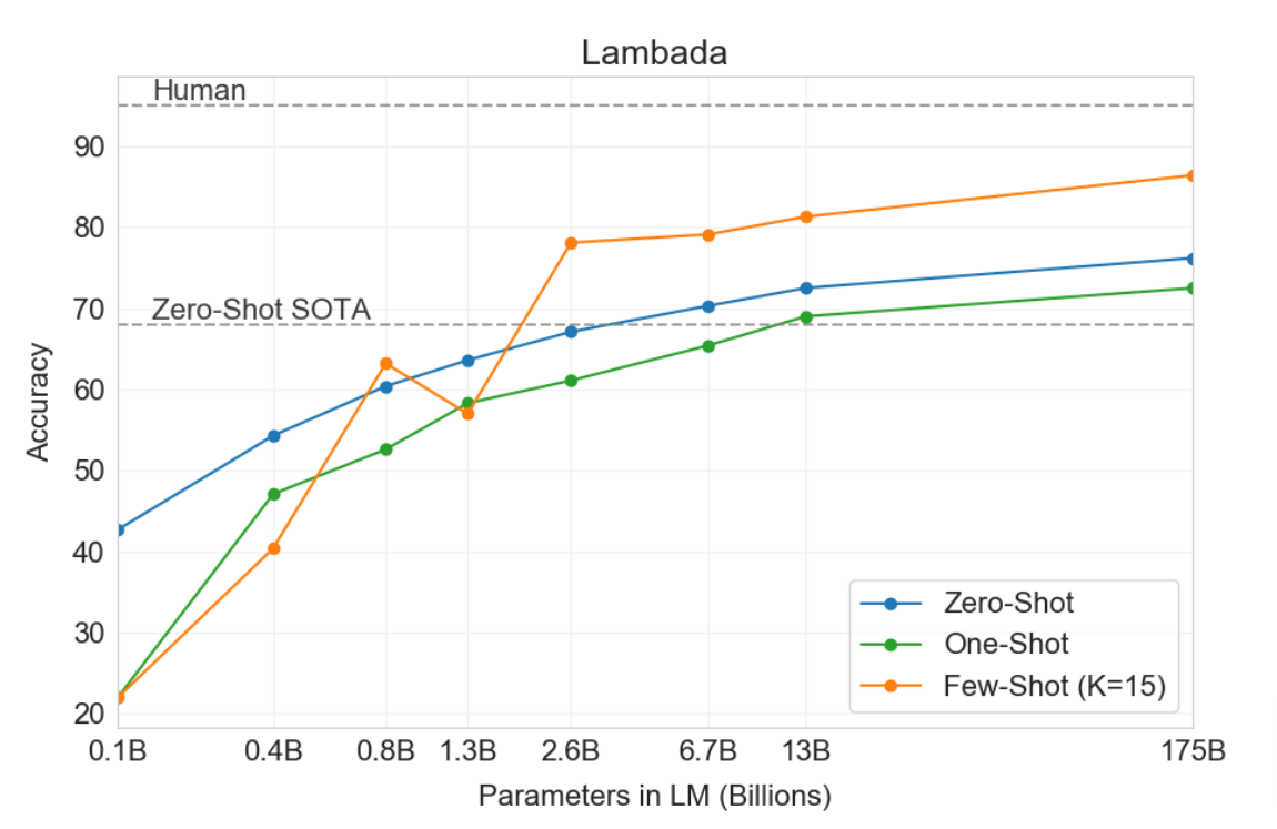
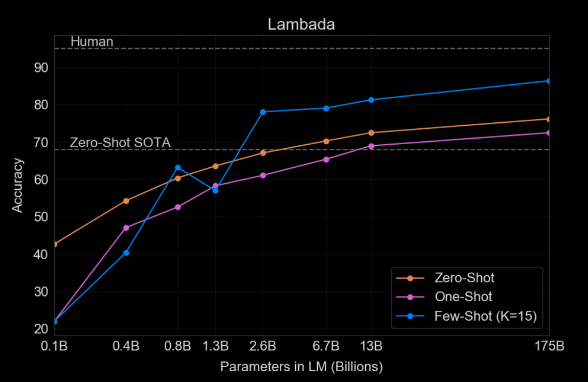
This graph on the left is from the GPT-3 paper [12], and it’s one of several that demonstrate that as the number of parameters in a language model increases, so does its zero-shot performance on downstream tasks. This graph, and many others like it, has occupied the interest of the language modeling community for the last five years. It really changed the way we think about many different problems and how we build, design, scale, and invest in models. Spoiler alert:… Bigger is better…sighs In fact, right now, it’s safe to say that there are nuclear power plants being built just to support this graph.
For an influential work on scaling laws, see [13].
Train vs. Test: When to spend your compute?
Recently, OpenAI released a new graph. Given the impact of their previous ones, we probably shouldn’t overlook this one.
In this graph (below), on the left-hand side, we see a curve that looks pretty similar to the curve we’ve seen before - more training compute leads to consistently better accuracy on a hard task. On the right-hand side, we see their latest plot. This curve looks similar in that we’re seeing compute contrasted with the performance of the model. What’s different is that this curve is showing test time compute. And what we are seeing is the performance on this task get much better as we add more test time compute to the system. This is new. We haven’t seen this before in language modeling, and it’s a topic of great interest.
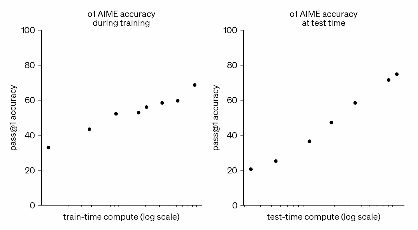
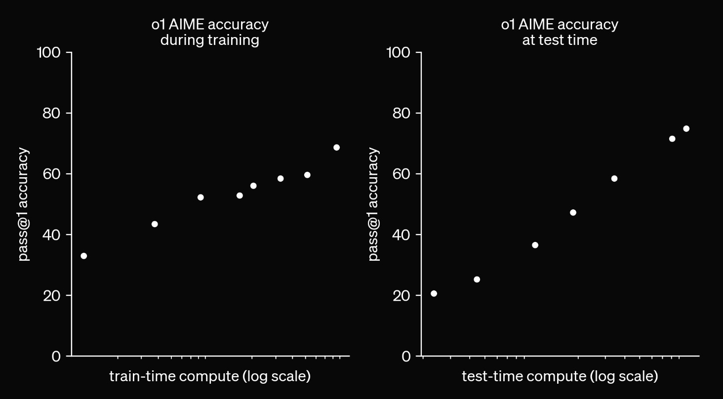
Our large-scale reinforcement learning algorithm teaches the model how to think productively using its chain of thought in a highly data-efficient training process. We have found that the performance of o1 consistently improves with more reinforcement learning (train-time compute) and with more time spent thinking (test-time compute). The constraints on scaling this approach differ substantially from those of LLM pretraining, and we are continuing to investigate them. … Similar to how a human may think for a long time before responding to a difficult question, o1 uses a chain of thought when attempting to solve a problem. Through reinforcement learning, o1 learns to hone its chain of thought and refine the strategies it uses. It learns to recognize and correct its mistakes. It learns to break down tricky steps into simpler ones. It learns to try a different approach when the current one isn’t working. This process dramatically improves the model’s ability to reason. To illustrate this leap forward, we showcase the chain of thought from o1-preview on several difficult problems below.
Why does this matter?:
If you are reading this around the end of 2024, then you’ve likely been exposed to numerous high profile comments/news about neural scaling “hitting a wall,” and the increasing internal pressure to deliver models that significantly outperform the current generation of models. However, it seems like several researchers, including o1 contributors, have been pushing against these claims (see Author Discussion). Or at least that the headlines are not telling the full story, and that while pretraining scaling may be producing diminishing returns, there’s a whole domain (test-time) that has yet to be fully explored.
Context: The Bitter Lesson
How did we get here?
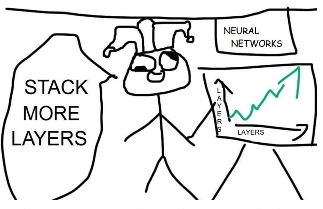
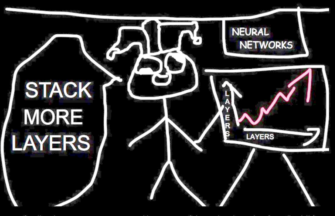
Most have already heard of the bitter lesson, but it’s worth revisiting because it helps explain why we care so much about scaling characteristics of models and compute in the first place.
Briefly, the bitter lessons emphasizes that simple and generalizable algorithms at scale will win over hand-crafted, “clever” solutions almost every time.
The bitter lesson is based on the historical observations that:
- AI researchers have often tried to build knowledge into their agents.
- This always helps in the short term, and is personally satisfying to the researcher.
- BUT, in the long run it plateaus and even inhibits further progress.
- Breakthrough progress eventually arrives by an opposing approach based on scaling computation by search and learning.
The bitter lesson is very frequently cited in the context of justifying scaling compute, and has likely contributed to the phenomenon of $100M+ single training runs we see today.
Context: Importance of Search
Compared to the attention scaling has received, the search component of the bitter lesson has been relatively underappreciated in the context of scaling up AI systems. However, what we might be seeing now is a move towards search, in particular, a type of search that is facilitated by learning to allow us to scale on some of these more technical problems.
Noam Brown, a researcher at OpenAI and contributor to o1, recently shared some thoughts on this topic:

The most important [lesson] is that I and other researchers simply didn’t know how much of a difference scaling up search would make. If I had seen those scaling results at the start of my PhD, I would have shifted to researching search algorithms for poker much sooner and we probably would have gotten superhuman poker bots much sooner.
While he’s referring to his work in the context of game playing and poker, his overall objective appears to be encouraging a shift towards thinking about search more.
Another lesser-known although influential paper, [15] discusses scaling laws for board games, where it is relatively easy to move back and forth between training and test-time search. Their main result that the performance achievable with a fixed amount of compute degrades predictably as the game gets larger and harder. But perhaps their secondary result (unbeknownst at the time) mayThe plots derived from the paper (below) show that the test-time and train-time compute available to an agent can be traded off while maintaining performance.
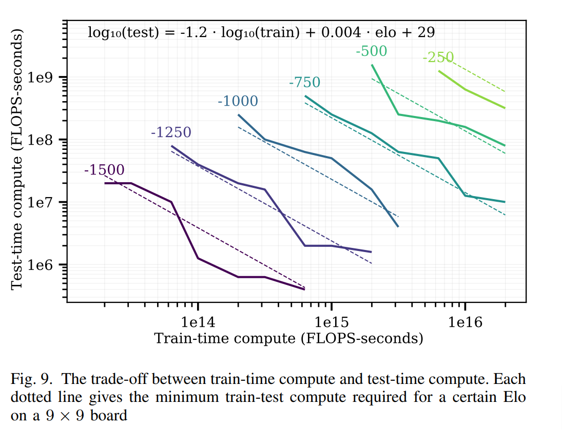
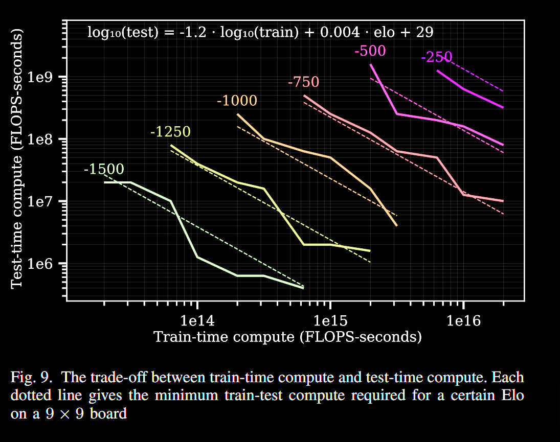
Remark: given the nature of the experiments, scaling laws plots are almost always shown on a log-log scale. What’s interesting about the plot above is that the amount of train-time compute considered is many, many orders of magnitude higher then the levels of test-time compute. While train-time compute is heavily amortized (because you only need to do it one time), there is a strong feeling that investing in test-time compute may provide much better “bang-for-your-buck”, especially in a regime where scaling pretraining is starting to produce diminishing returns
Review
When talking about similar techniques for language models, I think it’s helpful to consider the convergence of two research ideas:
- Chain-of-Thought reasoning: a technique that allows models to think before they speak, and is a form of search.
- Learned Verifiers & Reward Models: auxiliary models that help guide the main model towards better solutions by providing feedback scores on good vs. bad responses.
Chain-of-Thought
The origins of “Chain-of-thought” reasoning stem largely from increasingly sophisticated prompting techniques that enable/encourage LLMs to “verbalize” their thought process as output tokens before providing a final answer. This has been shown to increase performance on reasoning centric evaluations. Notable papers include:
- Self-Consistency [16] Majority voting of LLM output improves a bit.
- Scratchpad [17] / Chain-of-Thought [18] Can an LLM talk to itself and get better?
- Tree-of-Thought [19] Wouldn’t it be cool if you could scale this as a tree?
To see an a simple example of chain-of-thought reasoning, consider the following problem:
- The model is provided with a question as initial context - The model is prompted to generate intermediate steps in the reasoning process. - These steps provide a scratchpad for technical reasoning, allowing the model to “think” before it “speaks.”
Question: 4 baskets. 3 have 9 apples, 15 oranges, 14 bananas each. 4th has 2 less of each. Total fruits?
Let’s solve this step-by-step:
Fruits in one of first 3 baskets: 9 + 15 + 14 = 38
Total in first 3 baskets: 38 * 3 = 114
4th basket: (9-2) + (15-2) + (14-2) = 32
Total fruits: 114 + 32 = 146
Answer: 146 fruits
The example above is just meant to give you an idea of what chain-of-thought reasoning looks like in practice. We’ll later cover some examples of o1’s chain-of-thought reasoning as well as some of the techniques used to train models to think in this way.
Search Against Learned Verifiers
Another paper people often bring up a paper from OpenAI from 2021 [20]. In this paper, they train what we’ll call a learned verifier.
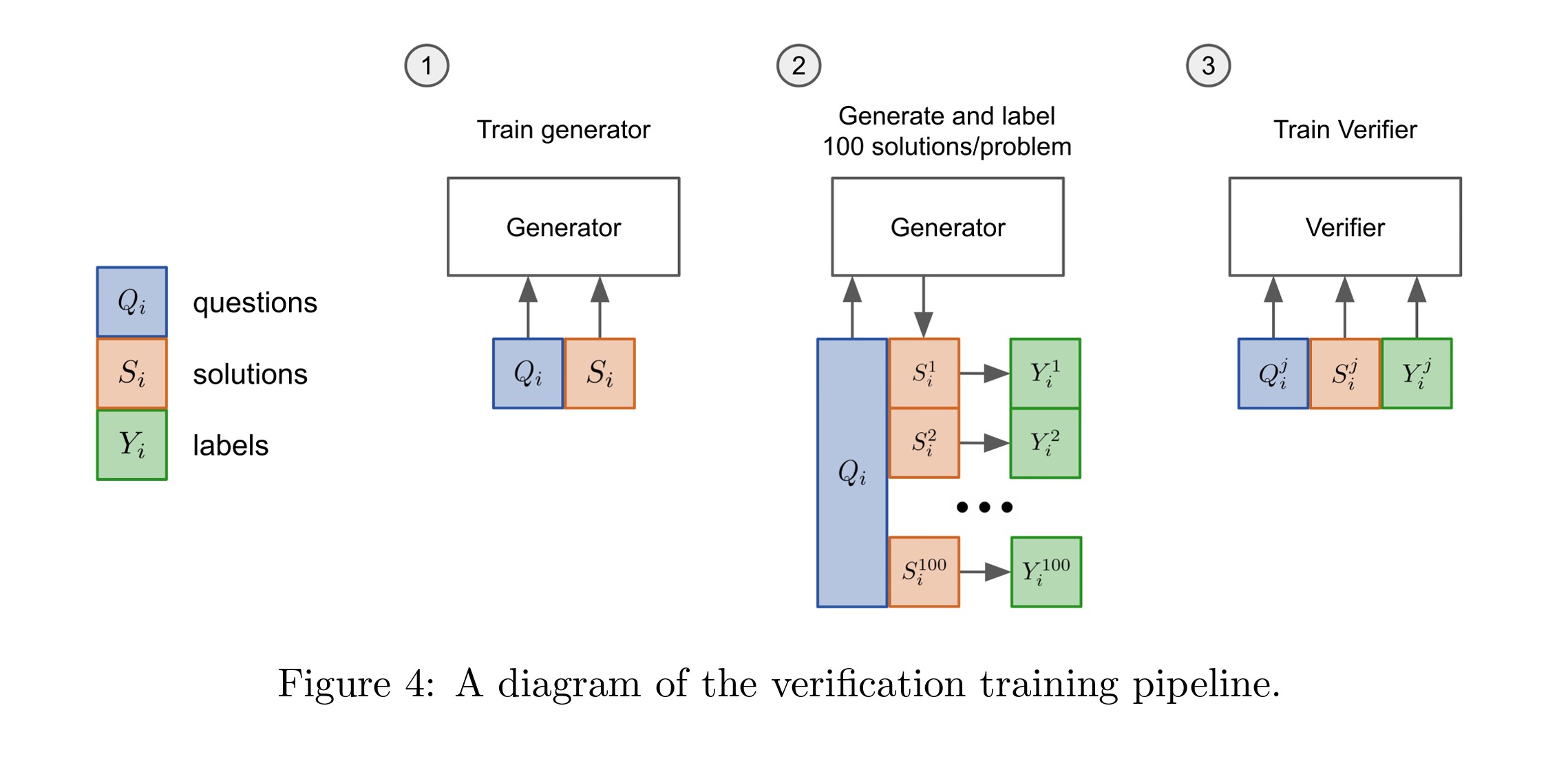
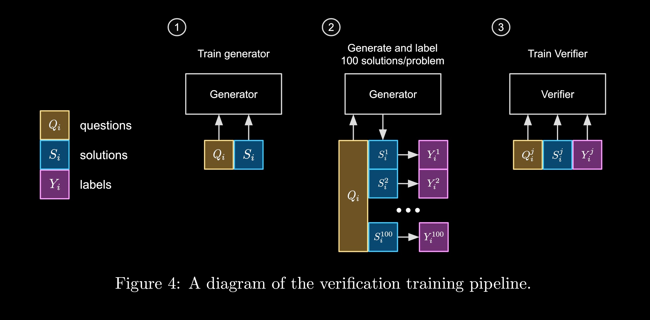
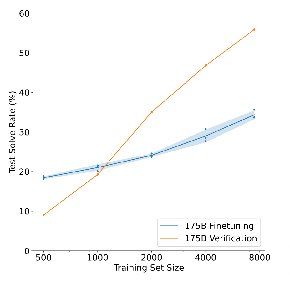
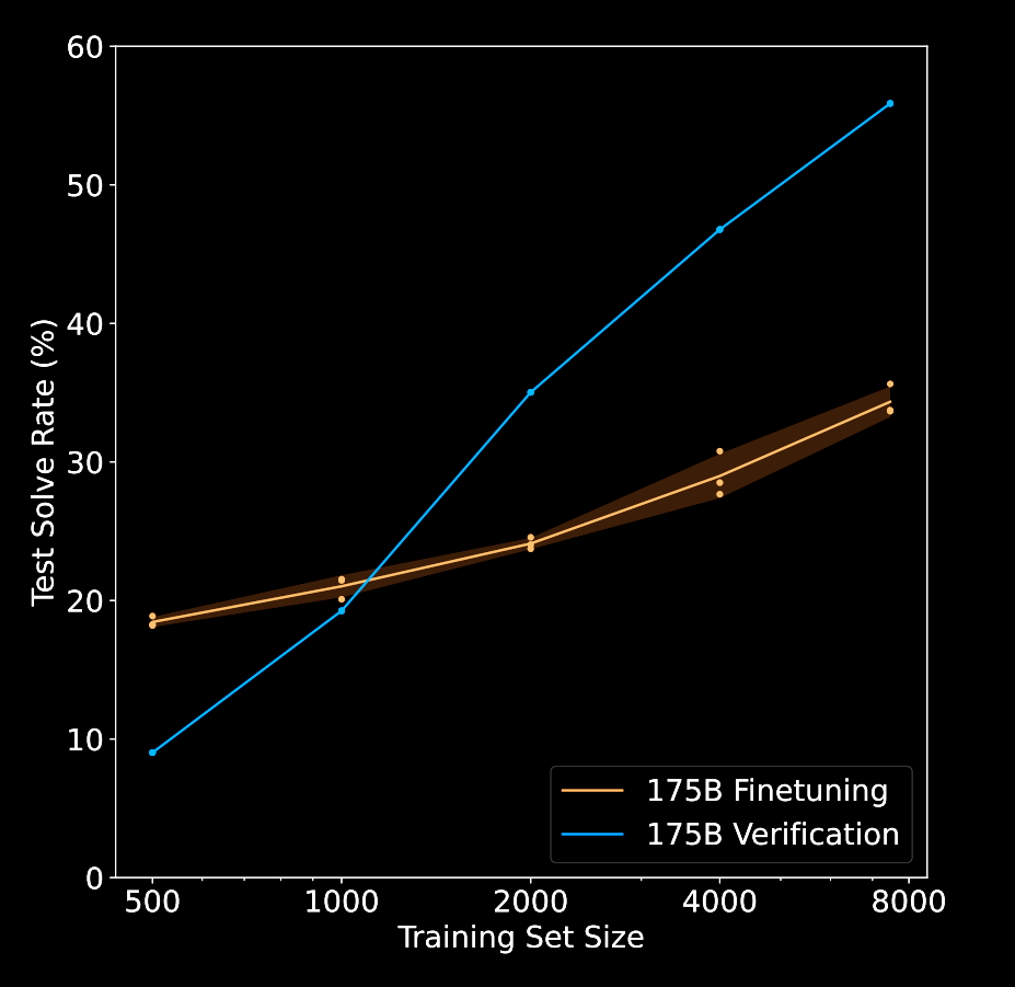
Figure 1: The verifier pipeline from [20]. The verifier is trained to score the quality of a generated trajectory. The verifier is then used to search for better trajectories.
To do this, they
- Train a generative model to produce an answer given an initial question.
- Use a generative model to produce hundreds of different candidate solutions, which are then annotated by experts as right or wrong.
- Using these annotations, they can then train a verifier. This verifier tells you if you’re doing well on the problem and can be used at test time to try to improve your answers.
While there are a lot of details to the paper itself, one of the most important results is they show that searching against this learned verifier can lead to improvements even upon just training on the actual good answers themselves. In the graph on the right, the steeper line shows the accuracy of the model that is running against the verifier compared to a model that’s just trained on the trajectories themselves. This is an argument for moving beyond the standard supervised fine-tuning, or SFT, more to a system that utilizes a learned verifier in order to inject new signal into the model.
This allows you to utilize that verifier to improve the model at test time. As we’ll see, we don’t think this is exactly what OpenAI is doing, but it gives you a sense of how they were exploring early uses of test-time compute in developing their systems. Don’t worry if you don’t understand all of the details yet. We’ll unpack them throughout the rest of this post.
The Clues
o1 Description
To gather clues about how o1 works behind the curtain, let’s first turn to OpenAI’s own words. The first informative sentence from their blog post is:
Our large-scale reinforcement learning algorithm teaches the model how to think productively using its chain of thought in a highly data-efficient training process.
Implication
This sentence gives us three clues into what might be happening:
- RL: Signal from verifiable problems
- CoT: Test-time occurs in token stream
- Data-Efficient: Bounded set of problems
We know the system is using reinforcement learning. The precise definition of reinforcement learning has become quite nebulous, and it means different things to different people. I think a fair operational definition in this context is that the model learns against some signal that comes from a “verifiable” problem. That is, there is some way to score the model’s output and this score does not come from purely supervised data.
Secondly, the method uses chain of thought. Specifically, it’s using chain of thought as its method of increasing test time compute. What this means is that we’re not doing any sort of search during test time. Instead, the system is just generating a very long output stream and using that to make its final prediction. In fact, we know this because OpenAI has been hesitant to release the internal CoT stream for a number of listed reasons, including competitive advantage.
Finally, the system is data efficient. What this means is that it’s learned from a relatively small set of data examples. This is not making any claim about compute or parameter efficiency or even parameter efficiency, just that the amount of actual problems it needs is relatively small, where relative here is compared to, say, training on the entire internet.
Current Assumptions
In addition to this sentence, there are several other assumptions that people seem to be making about these models:
- Single final language model with coherent CoT - the model just talks to itself until it thinks it has the right answer.
- Not following from expert examples/demonstration - it’s not just learning to copy human chain of thought examples, but from some other supervision signal, which may still involve human data.
- Behaviors are learned - they emerge somehow from data or self-play, but not from being given to the model explicitly.
o1 Chain of Thought
In the same blog post, OpenAI highlights this use of chain of thought.
o1 learns to hone its chain of thought and refine the strategies it uses. It learns to recognize and correct its mistakes. It learns to break down tricky steps into simpler ones. It learns to try a different approach when the current one isn’t working.
While this doesn’t tell us a whole lot of detail, it does further emphasize that the CoT is really where all the work is happening. Unlike other systems that build in complex search as part of their test time, this model is simply utilizing the chain of thought to do these steps as it goes. In some sense, they have linearized the search process in a way that continues to leverage the magic of transformer sequence models.
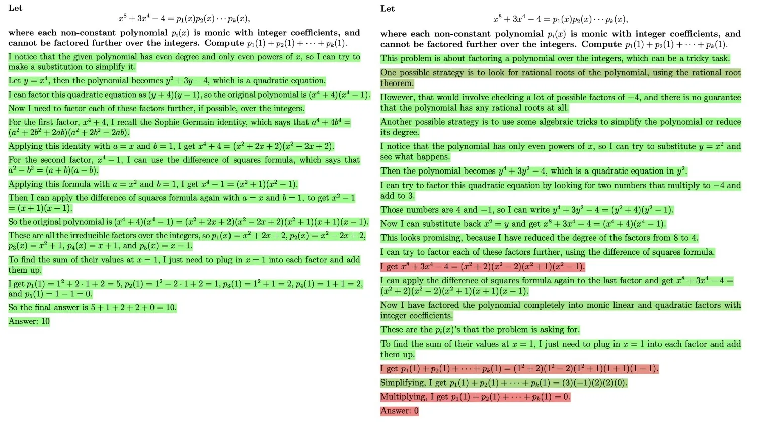
In their blog post, OpenAI additionally included some examples of the chain of thought for the system. You’re not actually able to see this chain of thought in the model they released, but we can look at some of the chains they provided. It highlights several emergent behaviors that the model has learned to do.
o1 CoT: Outlining
Implementation Outline:
- Capture input string as argument.
- Remove any spaces (if any).
- Parse input string to extract numbers as arrays.
- Since the input is in the format ‘[1,2],[3,4]’, we can:
- Remove outer brackets if necessary.
- Split the string by ’],’ to get each row.
- For each row, remove ’[’ and ’]’, then split by ’,’ to get elements.
- Build a 2D array in bash (arrays containing arrays).
First off, we can see the chain of thought for our programming problem. Just to note again, this is something the model itself produced in the process of solving the problem. What we can see is that the model has produced an outline of all the steps it would like to produce. The outline is numbered and includes complex sub-steps. If you read the rest of the chain of thought, you can see that it’s following this outline in the process of producing its answer.
o1 CoT: Planning
First, the cipher seems connected to the plaintext.
Given the time constraints, perhaps the easiest way is to try to see patterns.
Option 1: Try to find mapping from letters to letters.
Do any letters match?
First, let’s write down the ciphertext and plaintext letters on top of each other.
In another example, there’s a form of rudimentary planning. We can see that the system is aware of the time constraints it needs to answer the problem. It also is able to stop and propose different options and choose which of these it would like to follow. While this is all in English, it’s using cues like first or option one in order to specify the intermediate steps.
o1 CoT: Backtracking
Another ability that we see in these chains is forms of backtracking.
Similarly, m(x)* (-x 2) = (-x2n + 2 + m2n-2x2n + lower terms)m(x) * (-x 2) = (-x 2n + 2 + m 2n-2 x 2n + lower terms).
Wait, actually, this may not help us directly without specific terms. An alternative is to consider the known polynomials.
So m(x) = k ...
In this math example, it describes some intermediate term that it might need to compute. It then stops in the middle and says, “well, actually, this may not help us directly.” And then it proceeds to consider a different approach. This allows the model to go back and determine that it might want to say something different. Again, this looks a bit like search, but it’s not actually being performed with traditional search. It’s simply the model talking to itself in order to determine the answer.
o1 CoT: Self-Evaluation
A final ability OpenAI highlighted is something like self-evaluation.
Let’s analyze each option.
Option A: “because appetite regulation is a field of staggering complexity.”
Is that a good explanation? Hmm.
Option B: “because researchers seldom ask the right questions.”
Does this make sense with the main clause?
Here, the model says, “let’s analyze each option.” It then specifies the options it might want to consider, and it asks itself, is that a good explanation? The answer is a bit informal. It says, hmm, and then goes on to the next option itself. But again, this is an ability that can be used by the model in order to explore different possibilities and determine which ones might make sense.
Summary
So in summary:
- CoT provides test-time scaling
- CoT looks like search / planning in a classical sense, but is actually just talking to itself
- RL needed to induce this behavior
How does it learn to do this? Well, this is the big mystery!!
Technical Background
To get there though, we’re going to need some technical background. So in this section, we’re just going to focus on formalizing this idea of chain of thought. We’re not going to do any learning, but simply talk about what it means to start from a question, go through say four or five steps of intermediate reasoning, and then come up with an answer. For a full treatment of this topic, see [21].
Preliminaries
We’ll assume basic familiarity with autoregressive models and the language modeling objective. If you’re not familiar with these concepts, you can expand the section below to get a quick refresher.
Autoregressive Language Models
An autoregressive language model parameterized by that generates an output sequence conditioned on an input sequence is defined as:
with the convention that and . For ease of notation, we define , and may drop when it is clear from context. For a vocabulary size , the probability of prediction the th token , , is computed using a softmax with temperature on logit scores of all the tokens: , where . Higher values of temperature introduce more randomness, while setting temperature makes the output deterministic, corresponding to greedy decoding.
Language Modeling Objective (Next-token prediction)
During pretraining and (supervised) fine-tuning (SFT), the learning objective minimizes the cross-entropy loss between the model’s predicted next token distribution and the ground-truth token distribution. Given a dataset of input context and target sequence , the objective is to minimize the negative log-likelihood of the target sequence given the input context :
Stepwise CoT Sampling
In the section above, we considered the standard language modeling objective, which operates on a per-token basis. However, in the context of chain of thought, it’s more useful to thinking in terms of steps in the chain, where each step is almost always composed of multiple tokens. So, at the risk of overloading our notation, we’ll abstract a bit away from the fact that this is a language model, and just think about it producing steps along in this chain.
Let’s revisit the CoT example from earlier:
- : problem specification
- ; chain of thought (CoT) steps - not individual words, but instead full steps (1, 2, 3,…)
- ; final answer
- Note: , and are now all sequences of tokens!!
- is step index, not token index
Question: 4 baskets. 3 have 9 apples, 15 oranges, 14 bananas each. 4th has 2 less of each. Total fruits?
1. Let’s solve this step-by-step:
2. Fruits in one of first 3 baskets: 9 + 15 + 14 = 38
3. Total in first 3 baskets: 38 * 3 = 114
4. 4th basket: (9-2) + (15-2) + (14-2) = 32
5. Total fruits: 114 + 32 = 146
Answer: 146 fruits
The final goal is to produce a distribution over answers conditioned on our input . This distribution is defined by taking an expectation over these latent chain of thought steps :
Warm-up: Ancestral Sampling
As a warm-up, let’s consider how standard chain of thought is done. We can’t actually compute the expectation over all possible intermediate steps, so instead we run “ancestral” sampling. This is a fancy term that just means let the language model generate until it produces an answer.
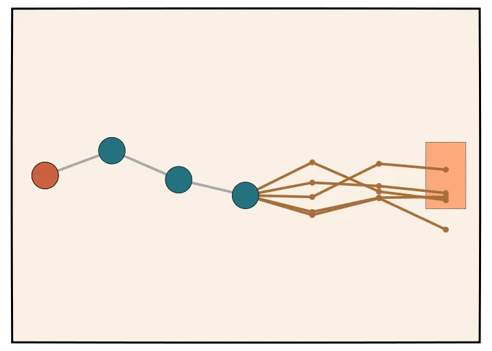
Specifically we’ll sample steps , these are represented by the green dots in the figure picture, until we get to an answer represented by the dot on the right.
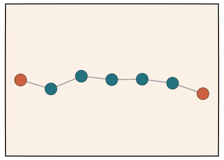
Above, is the total amount of test-time compute. Note: In this regime, there’s not really a clean and reliable way to increase the value of for a single sampling. Without additional prompting, the model likely will arrive at its final answer “when its going to arrive.”
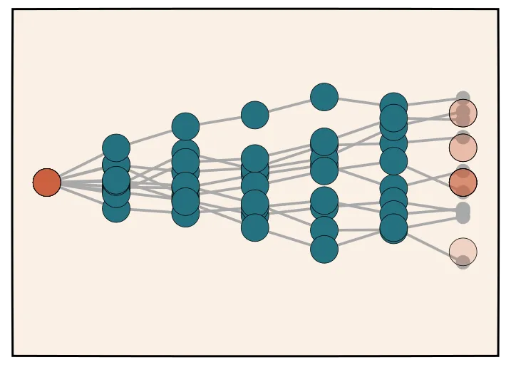
Self-Consistency / Majority Vote
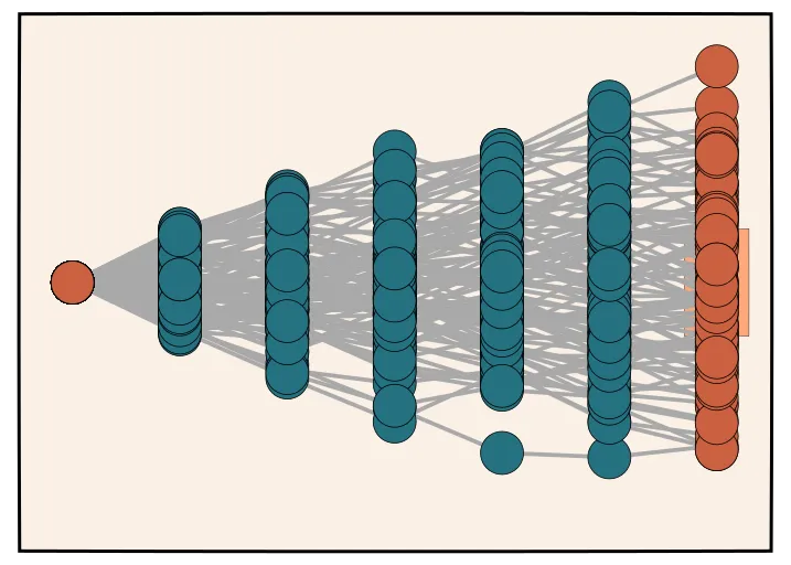
Many papers, such as [16], have noted that there is a way to get better answers to these problems. Instead of taking a single chain of thought and using it to produce the answer, we can instead sample chain of thoughts. Once we have these different chain of thoughts, we can take a majority vote in order to determine the majority answer. In this diagram here, each one of these chain of thoughts is sampled independently, and then we do some sort of normalization. The answers that are most common are the ones we decide. This provides a strong baseline and a way to utilize more test time compute to slightly improve our answers.
For samples,
Pick majority choice
You can obviously do this to a large extent, but people have found that it doesn’t lead to some of the amazing results that we’re seeing in the o1 blog post.
Assumption: Automatic Verifier at Training [3]
The second piece of machinery we need is a “verifier.” Explicitly, we’ll assume that we have an automatic verifier, but we only have it at training time. We’ll define this automatic verifier as taking some answer why and telling us if it is right or wrong.
Common Verifiers/Datasets:
- Regular expression for math [20]: Extracts and parses numerical or symbolic answers from text, (e.g., “Boxed” LaTex answers) and compares them to the ground truth.
- Unit test for code [22]: Compiles and runs unit-test code snippets provided by the model and checks pass-rate.
- Test questions for science [23]
Again, just to reiterate, we don’t have this at test time, but we are going to utilize it as a way to provide training signal for us to produce a better model.
Automatic Verifier?
By “automatic,” we really just mean that it is some sort of procedure (e.g., like a python function) that can take an answer and tell us if it’s right or wrong. In other words, it isn’t a human annotator nor is it a learned model.
It’s not clear whether OpenAI is actually utilizing automatic verifiers or whether they are using learned verifiers. It may likely be a combination of both. In some of their papers, they explicitly try to learn verifiers for some technical problems. Their argument is that this can produce more general-purpose models, and it’s a way for them to utilize their large annotation facilities in order to improve their models.
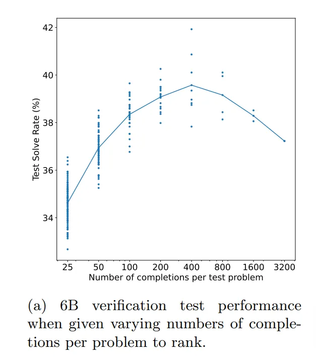
In the case of learned verifiers, there are some interesting research challenges. For instance, one challenge is that with a learned verifier, if the generator produces, say, wild solutions, sometimes the learned verifier gets confused and accepts them. In this graph on the right, they show that for a math problem, the model will continue getting better, but then it will plateau and even get worse as they take more samples. They discuss how this is a challenge with a learned verifier, and I have to assume they’ve collected a lot of data and thought about this problem a lot more in recent years.
Rejection Sampling Best-of-N
If you are fortunate enough to have an automatic verifier, there are several ways of using it to improve your performance. One method is to do rejection sampling, and is the approach taken in [20].
This approach is similar to majority voting - you simply sample different chain of thoughts - but then you use your verifier to determine which of these are correct. This process may be extremely compute intensive, but it does provide a way to obtain good chains of thoughts that lead to verified solutions.
For to :
Verified set
Note: For very difficult problems, it’s not guaranteed that the model will every yield correct solutions, even for large .
Monte-Carlo Roll-Outs
Perhaps we want to be a bit more systematic in our approach and estimate the strength of particular intermediate step. Here, apply the same process as rejection sampling, but starting from an intermediate CoT step. From the intermediate step, we can compute “rollouts”
Given partial CoT , expected value,
Monte Carlo for this expectation.
Goal: Learning with Latent CoTs
Now, given this background, we come to our main goal. We would like to learn a model that can take into account these latent chain of thoughts. We can write this down explicitly as a maximum likelihood problem, where we are interested in learning the model that performs as well as it can at producing verified solutions:
Maximum likelihood;
Marginalizing over all possible chains of thoughts that lead to correct solutions is combinatorially intractable.
Reinforcement Learning
Important practical choices
- Batched? → Compute trajectories first, then train
- On-policy? → Sample from current model
- KL Constraints on learning.
- Specific algorithm choice (REINFORCE, PPO, etc)


When training a model for reasoning, one thing that immediately jumps to mind is to have humans write out their thought process and train on that. When we saw that if you train the model using RL to generate and hone its own chain of thoughts it can do even better than having humans write chains of thought for it. That was the “Aha!” moment that you could really scale this. — Building OpenAI o1 (Extended Cut)
The “Suspects”
Following [1], I think it is reasonable to narrow down the possible techniques that OpenAI is using to improve their reasoning model into several “suspects”:
Suspect 1: Guess + Check
Suspect 1 is the simplest. You might also call this a “Propose and Critique” loop. In essence, it is just like rejection sampling where you then train the model on the good samples it produces; thus, it is seen as a form of self-training.
Framework: Rejection Sampling Expectation Maximization
As you’d expect, it consists of three steps:
- Sample CoTs
- Use verifier to check if successful
- Train on good ones
The goal:
- E-Step: For to :
Keep verified set
- M-Step: Fit
We can think about this as a form of rejection sampling expectation maximization. EM is a very traditional algorithm in machine learning and it’s been applied to these sort of reinforcement learning algorithms for decades.
We can think of the expectation step (e-step) as running rejection sampling and the maximization step (m-step) as fitting the language models to samples that fit with our posterior. The more we run this expectation step, the closer to the true expectations we’ve calculated, and the better our end step will in getting to the answer itself.
Variants
This approach has been explored numerous times over the years, and so it goes by different names in different areas. OpenAI refers to it as best-of- training. Recent popular variants include:
- Expert Iteration [24] Search, collect, train. Method for self-improvement in RL.
- Self-Training [25] Classic unsupervised method: generate, prune, retrain
- STaR [26] Formulates LLM improvement as retraining on rationales that lead to correct answers. Justified as approximate policy gradient.
- ReST [27] Models improvement as offline-RL. Samples trajectories, grow corpus retrain.
- ReST-EM [28] Formalizes similar methods as EM for RL. Applies to reasoning.
- Filtered Rejection Sampling [29] Used rejection-sampling against a reward model in a web-browser based environment.
Empirical Results
At a high level, all these papers come to a similar conclusion. This method is simple, but it works, and it works pretty well. You can get relatively consistent improvements, particularly in lower samples, across many different problems (and thus, should probably be a required baselines for most papers in this space).
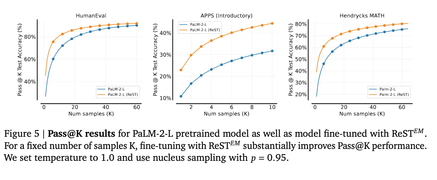
Empirical results from ReST paper [28] demonstrating improvements over the baseline PaLM-2-L pretrained baseline.
Reminder: These methods are concerned with self-training of the generator model, not a verifier (because they use automatic verifiers). The generators are trained on their own solutions that have been verified as correct by the verifier (and in these work ignore incorrect solutions). Try to keep this in mind as we move forward because there’s a lot of overlap between these (and upcoming) methods.
Learned Verifier
Of course, the assumption with the above is that we have access to the verifier. It’s not clear exactly how you could productively increase test-time compute if you only had an automatic verifier during training.
Since we have a lot of samples from rejection sampling, one idea would be train some sort of learned verifier that we can keep around test time. We could then use this as part of chain of thought or for some sort of test time rejection sampling.
How do you train a learned verifier?
Descriminative Verifiers
The predominant approach to training verifiers for reasoning is to fine-tune an LLM classifier on a dataset of correct and incorrect solutions generated from a fixed LLM, producing a scalar reward to score the solution given the problem , and thus does not utilize any of the underlying generative capabilities of the pretrained LLM.
Given a reward-modeling (RM) dataset , we can define the verifier objective as:
where ), , is a special token, and and are correct and incorrect solutions, respectively.
Note: Here, I’ve explicitly used the term “discriminative” in order to distinguish from the “generative” verifiers that are used in the next section. Additionally, the terms “learned verifiers” and “reward models” are used somewhat interchangeably because they are functionally similar, but the former is typically used in the context of test-time verification, while the latter is used in the context of training-time reinforcement learning.
Combining Learned Verifiers with Self-training
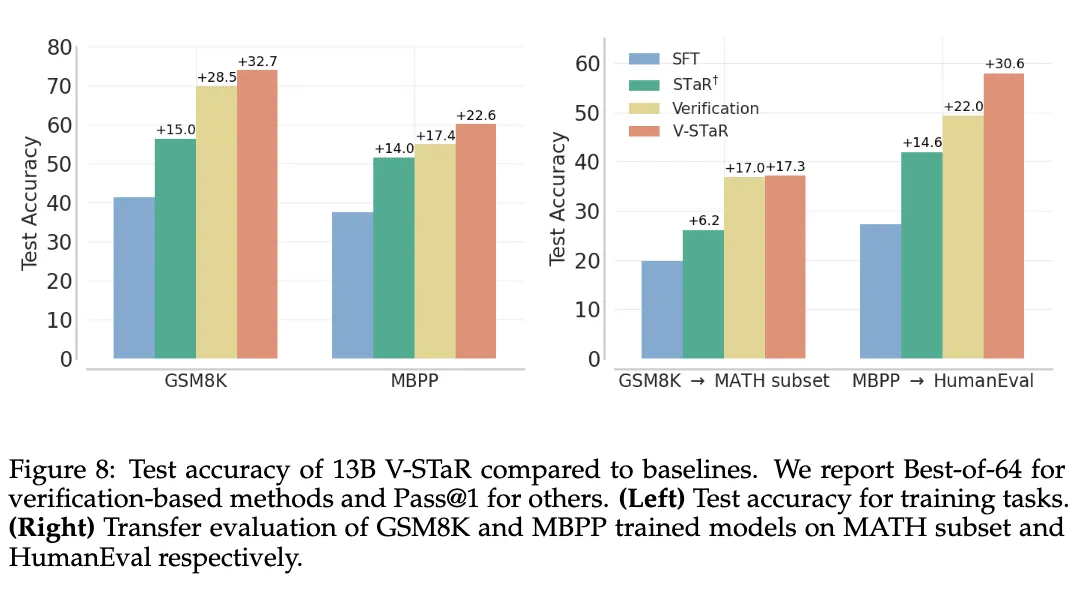
As noted by a recent paper, “Verification for Self-Taught Reasoners” (V-STaR) [30], common rejection-sampling approaches discard large amounts of generated incorrect solutions and only use the correct ones for self-training, potentially neglecting valuable information in such solutions. The key idea behind this work is to utilize both the correct and incorrect LLM-generated solutions during the iterative self-improvement process to train a verifier using DPO, in addition to training a LLM generator using correct solutions. They propose utilizing both the correct and incorrect solutions generated during the self-improvement process to train a learned verifier using DPO that judges correctness of model-generated solutions. This verifier is used at inference time to select one solution among many candidate solutions. We may see additional papers in the future that explore this direction.
V-STaR consists of the following steps:
- Fine-tune a pretrained LLM on the original training dataset to obtain a generator .
- Sample completions for each problem in the training data from the generator , where .
- Generated solutions are labeled for their correctness using ground truth answers or test-cases.
- Only correct completions are added to the generator training data as
- Both correct and incorrect completions are added to the verifier training data as so the verifier can learn from the generator’s mistakes.
- In the next iteration , the generator is obtained by finetuning the pretrained model on the augmented dataset . The verifier is trained on the augmented dataset .
V-STaR: Training Verifiers with DPO
To use DPO for training verifiers, a preference pair dataset is constructed using collected solutions in , with correct solutions preferred over incorrect ones. Specifically, we have , where is the number of preference pairs generated from the Cartesian product of correct and incorrect solutions for each problem . The verifier using this dataset and the SFT policy using the DPO objective:
where is the sigmoid function, and is a hyper-parameter controlling the proximity to the reference policy .
The DPO objective steers the verifier towards increasing the likelihood of correct solutions and decreasing the likelihood of incorrect solutions for a problem . At inference, the likelihood of a generated solution given a problem under the trained DPO verifier i.e., ) is used as scores to rank candidate solutions.
Is this o1?
So is O1 just a guess and check RL system? Well, there’s some signs it might be, or at least that it’s using some of the same techniques. What are the pros and cons:
- ✓ Extremely simple and scalable - aligns well with OpenAI/Bitter Lesson’s approach to driving progress - just building larger and more powerful versions of things that already worked reasonably well
- ✓ Positive results in past work - by many groups including Google and OpenAI itself, which produces several important papers in this space
- × No evidence this learns to correct, plan, backtrack, etc. - Requires a fairly large leap of faith to believe that this simple method could produce the complex behaviors we see in the o1 blog post.
- × Computationally inefficient search - Sampling at a high temperature, as you might have to do in order to achieve a good diversity of samples, is likely to produce a large proportion of rejections.
Final verdict: Has the right spirit, but feels like it doesn’t quite have enough structure. Given OpenAI’s follow up work in this area, I think it’s likely to involve process-level supervision in some form, which we’ll discuss next.
Suspect 2: Process Rewards
In the previous section, we focused on verifiers that provide feedback to a generator only AFTER the model had produced a full solution. This is typically referred to as “outcome-supervised reward models” (ORM). But what if we could provide feedback during the generation process itself? This is the idea behind process rewards and it’s a natural extension of the previous section. The steps are as follows:
- During CoT sampling, use guidance to improve trajectories
- Check if final OR partial versions are successful
- Train on good ones
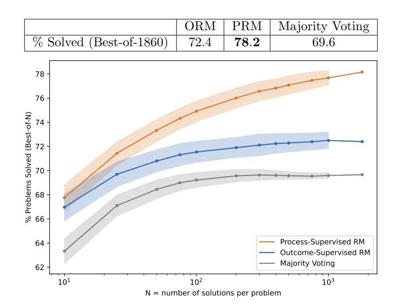
The term process rewards and process reward models (PRM) comes from two papers, one from Google [3] and one from OpenAI [4]. In these papers, they learn an early verification model, which they call a PRM or process reward model. They show that learning this intermediate model can improve in rejection sampling compared to a learned model that gets the full solution. The graph on the right compares the learned intermediate model both to majority voting and to a model learned only on full solutions.
- Early learned verification (PRM) improves over learned verification (ORM)
Note: this graph is not making any claim about the learning process, just that we’re able to successfully complete more CoTs by utilizing PRMs
Learned Process Rewards
There are several ways for parameterizing and acquiring this process reward model, which we explore now. For a brief primer on the training process reward models, see the expandable section below.
Training Process Reward Models
Let’s first revisit the ORM objective for a single example, which consists of the cross-entropy between the model’s prediction and the ground truth label:
where is a scalar value between 0 and 1 returned by the reward model, and if is correct and otherwise.
The PRM objective is similar, but instead produces a score for each step in the chain of thought, which are then summed the final loss for the entire chain of thought:
where , if is correct and otherwise, and is the number of steps in the chain of thought.
Human Annotations - Let’s Verify Step by Step [4]
One might simply be to sample trajectories from your model and utilize human annotators to label these. One effective approach to improving AI models is to use human annotators to evaluate the model’s outputs. This method, explored in the “Let’s Verify Step by Step” research, involves sampling trajectories from the model and having human experts label them.
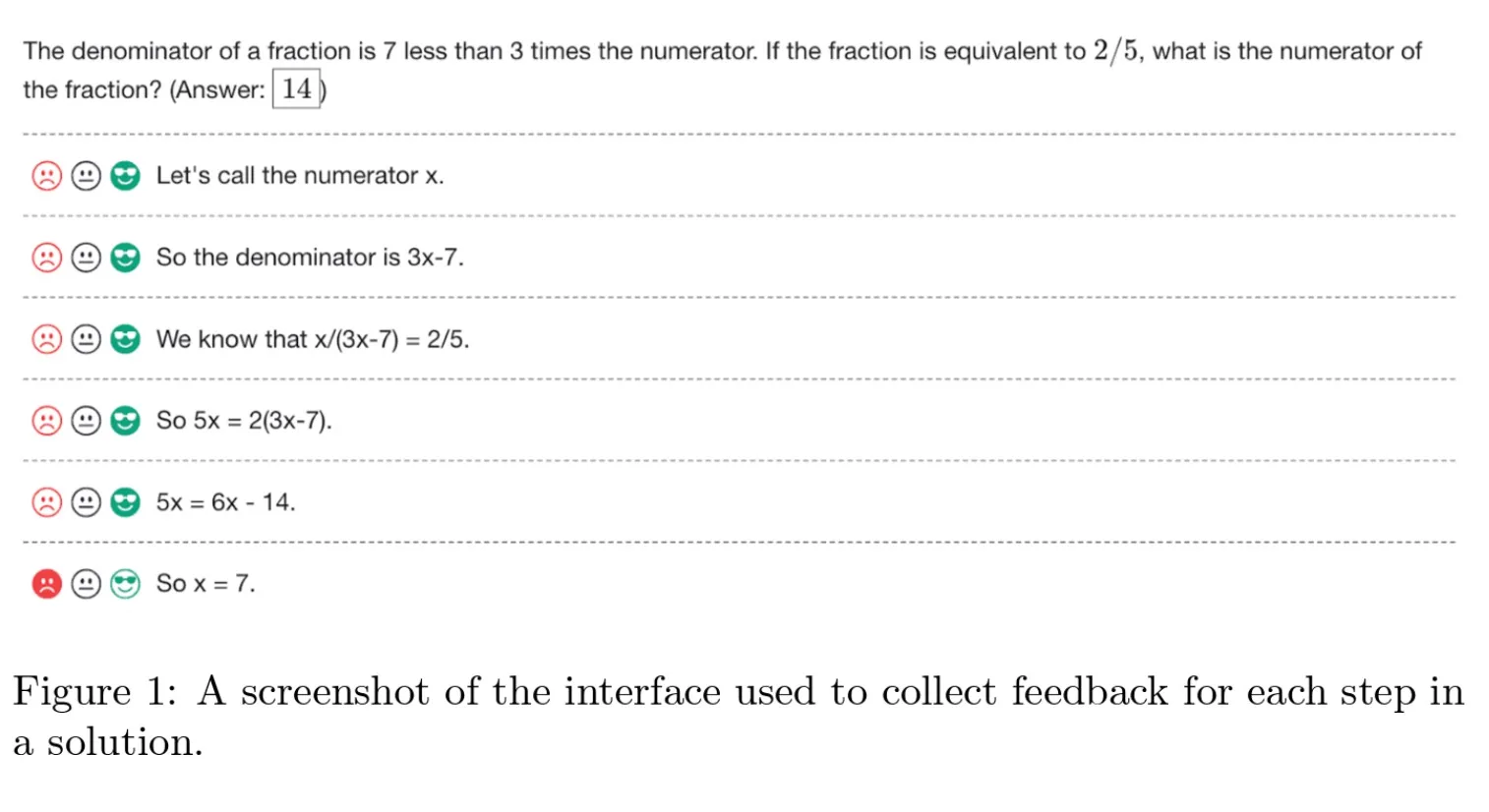
Data collection and PRM scoring from “Let’s Verify Step by Step” [4]
To collect process supervision data, human data-labelers were presented with step-by-step solutions to MATH problems sampled by the large-scale generator. Their task was to assign each step in the solution a label of positive, negative, or neutral, using the interface shown in the figure above. OpenAI released their “PRM800K” training set contains 800K step-level labels across 75K solutions to 12K problems.
Model Annotations: Math Wizardry with RLEIF [5]
An obvious bottleneck in the process reward model is the need for human annotations. It is very labor intensive to have humans label each step in a chain of thought for many problems. Since human annotated data is expensive to collect, an obvious question to ask if whether you can use a model to annotate the data for you. This is explored in the “Wizard” series of papers including WizardMath, which extends the use of PRM to improve open source models with fine-tuning for reasoning. Specifically, WizardMath used Llama2 as the base model, then applied their approach, Reinforcement Learning from Evol-Instruct Feedback (RLEIF), in order to fine-tune the model to handle complex math tasks.
Reinforcement Learning from Evol-Instruct Feedback (RLEIF) first uses Evol-Instruct to generate a variety of problems from a base set, then trains both an IRM (instruction reward model) and PRM (process-supervised reward model) to evaluate/reward the problem and the steps towards its solution. These policies are used for fine-tuning the LLM.
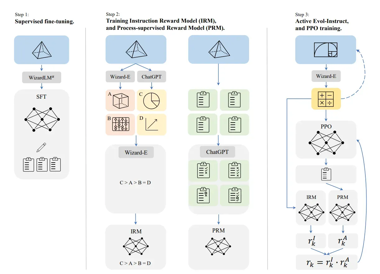
Apparent Limitation: Many of these work rely on using a stronger LLM, such as gpt-3.5 or gpt-4 to expand instructions, questions and provide process annotation to improve a smaller and/or less capable model. It’s not clear if this approach works for improving a model beyond the performance of the original LLM annotator model.
Automatic Process Annotation - MC Rollouts
More recently, there have been works, such as Math Shepherd [31], that estimate the quality of intermediate steps in a chain of thought without human or model-based annotations by leveraging Monte-Carlo rollouts. A key difference here is that the process-level data and annotations are generated from the same model they want to improve.
The key insight suggested by Math Shepherd is the following definition of the quality of a reasoning step:
the quality of a reasoning step is its potential to deduce the correct answer.
Intuitively, a good reasoning step should be one that more likely leads to the correct answer. If even after many repeated attempts, the correct answer cannot be reached from a particular reasoning step, then that step is likely not a good one.
The overall training process is as follows:
- For partial , rollout:
- Use Monte-Carlo to estimate step annotations
- Learn to approximate based on rollouts
There are a couple of points to note:
- Computing the full MC rollouts is computationally expensive, so this method is not suitable for real-time inference (training is done offline).
- At inference time, you can use the learned reward model to guide decoding with techniques such as beam search.
- If you do several iterations of self training, you can also use the learned reward model to guide the MC rollouts.
Automatic Process Annotation - Math Shepherd Details
In the Math Shepherd paper, they make some particular choices around how they do this process, so I include it here for completeness.
Automatic Process Annotation - MC Rollouts
To quantify and estimate the potential for a given reasoning step , subsequent rollouts are generated from that particular step: , where and are the decoded answer and the total number of steps for the -th rollout, respectively. The potential of the reasoning step is estimate in two ways:
- Soft Estimation: The potential of is estimated as the average of the verification scores of the rollouts (MC rollouts).
- Hard Estimation: Gives a binary estimate of the potential of based on the existence of a rollout that produces the correct answer.
Inference time: Ranking for Verification
Similar to [4], they use the minimum score across all steps to represent the final score assigned by the PRM to a solution The aggregate score for each
They show that in this model, they’re both able to find better solutions with their learned intermediate guide, and they’re also able to learn a final model that’s better at math.
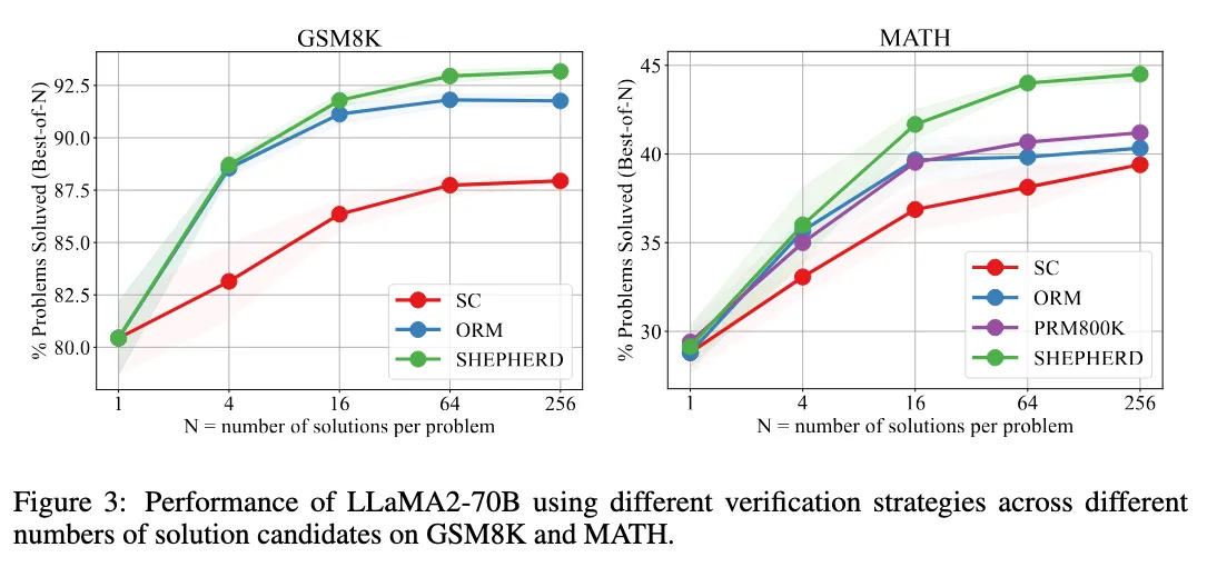
Math Shepherd: Verify and Reinforce LLMs Step-by-step without Human Annotations [31] showing the improvement of their method over other such as Self-consistency and Outcome Reward Models (ORMs).
This sort of ideas was also explored in the context of code generation: Let’s reward step by step: Step-Level reward model as the Navigators for Reasoning [32].
Generative Verifiers: Reward Modeling as Next-Token Prediction [6]
While LLM-based verifiers are typically trained as discriminative classifiers to score solutions, they do not utilize the text generation capabilities of LLMs. The idea here is to train verifiers using the standard language modeling objective, jointly on verification and solution generation. In this way, the reward model can itself use chain of thought. It might try to reason about individual steps and utilize them to decide upon the answer. What’s important about this step is this is an idea that merges the generator and the verifier. You can have a single model that is both trying to do reasoning and also trying to verify this reasoning.
This approach has the following advantages:
- these models integrate seamlessly with instruction tuning
- enable chain-of-thought reasoning for verification
- utilize additional test-time compute via majority voting for better verification
Generative Verifiers Method
Direct Verifier
In its simplest form, GenRM predicts whether a solution is correct using a single “Yes” or “No” token. This can be done by maximizing for the solutions in and for the solutions in .
where .
At inference, we use the likelihood of the “Yes” token as the verifier score: .
Unifying Generation and Verification
GenRM integrates reward modeling with SFT by training the data mixture in the SFT loss to include both verification and generation tasks. Given a verification dataset :
Altogether, these approaches start to bring the full story into a bit more focus. If we’re going to use a verifier that is also using chain of thought, and we’re going to merge that into a single stream, we can imagine alternating between generation and verification, and using that to improve our test-time solution.
Incorporating at Test-Time
As we discussed, the major advantage of a learned verifier is that we can use it at test time - we don’t need the original automatic verifier (which we aren’t allowed to use anyway). Moreover, if it is generative, then it can be merge into a singel CoT stream. Hints of this appear in the OpenAI blog post.
For example, if we look back at one of the o1-planning Cot, we see statements like, “Is that a good explanation?” While traditionally we would think of this as part of the generator, this might be part of a verifier that’s been merged into the same model. It can move back and forth between generation and verification within a single language model.
Is this o1?
So is this a one? Well, there’s some evidence for and against:
- ✓ Evidence that intermediate guides are effective
- ✓ Removes challenges of full/separate learned verifier
- × Not clear if this is enough for planning.
- × Need to combine generator / guide into one CoT
Overall, on the positive side, it does seem like this is a simple and effective approach that aligns both with the research papers that OpenAI is publishing and their broader strategy of embracing simple and scalable methods.
On the negative side, we haven’t really seen anything yet that explains some of the advanced planning that we’ve seen this model do. And we don’t really know how to fully do this combination of generator and process reward model into a single chain of thought. It’s a compelling idea, and that’s not to say that OpenAI hasn’t figured it out internally, but there are a lot of details and open questions that the broader research community hasn’t yet answered.
Final Verdict: If I had to guess, I would say I personally think this is probably closest to what we might expect o1 to be.
Suspect 3: Learning to Search in Language
In the previous sections, we have looked at various combinations of:
- using automatic verifiers at training time to generate self-training data
- using these generated samples to improve generators as well as learned verifiers, which can be used at test time
- training learned verifiers to provide feedback at the process/step level
- combining generation and verification into a single model
Aspects we did not cover in detail are methods for
- search: using these learned verifiers to guide the search process during generation allowing the model to explore the space of possible solutions more effectively.
- self-play: using the model to generate its own training data and learn from it.
LLM Search and Planning
Some relevant works to check out are:
- Stream of Search [7] Training on linearized, non-optimal search trajectories induces better search.
- DualFormer [33] Training on optimal reasoning traces with masked steps improves reasoning ability.
- AlphaZero-like [34] / MCTS-DPO [35] / Agent Q [36] Sketches out MCTS-style expert iteration for LLM planning.
- PAVs [37] Argues for advantage (PAV) function over value (PRM) for learning to search. Shows increase in search efficacy.
Reminder: AlphaZero
To prime this discussion, let’s remind ourselves of AlphaZero, the canonical example of self-learning This was a very important paper in the history of deep learning and RL. Here, they demonstrate that a system can be completely trained from scratch using self-play reinforcement learning and achieve expert-level performance. This method could be scaled without human data.
At a high level, the system is based on Expert Iteration combining learned model with expert search with a verifier:
- It plays games using a complex search algorithm (Monte Carlo Tree Search).
- Generate samples using , reward model , and search algorithm (e.g. beam search)
- Label samples using , which comes from the outcomes of the games
- Train , on the labeled trajectories.
- Repeat: It then uses that neural network to again play some more games.
There are several reasons this system is relevant to the discussion, but one of the more recent ones is this work on alpha proof. We don’t have a lot of details behind how AlphaProof works, just that it did extremely well at a very hard math competition, and a blog post that says, When presented with a problem, AlphaProof generates solution candidates and then proves or disproves them by searching over possible proof steps in Lean, which is a proof assistant, which is a proof assistant. Each proof that was found and verified is used to reinforce AlphaProof’s language model, enhancing its ability to solve subsequent more challenging problems. So if you squint, this does seem rather similar to some of the language we saw in OpenAI’s blog.
Framework: Beam Search with Guide
Here is the goal is to utilize the learned verifier
to guide the search process during generation.
For each step ,
- Sample many next steps,
- Keep the top samples, ordered by
Note: Beam search allows choosing lower ranked samples in the short term with the hope of finding a better overall solution in the long term,
MCTS for Language
MCTS is a more sophisticated search algorithm that has been used in games like Go and Chess. MCTS works to balance exploration and exploitation by sampling from the search space and then using a value function to guide the search towards more promising areas.
Briefly, the steps of MCTS are as follows:
- Selection : Walk down tree to leaf
- Expand : Sample next steps , pick one at random
- Rollouts : Sample steps
- Backprop : Update nodes counts and wins for parents
Since, we are fairly confident from rumors that, at present, OpenAI isn’t using MCTS at the moment, we’ll save the details for a later post!
Is this o1?
- ✓ Major demonstrated RL result
- ✓ Scales to more train-time search
- × Costly to maintain open states
- × More complex algorithmically
- × OpenAI comments / rumors
Suspect 4: Learning to Correct
Our final method is “learning to correct.” To motivate these algorithms, one should note some differences between game playing and language. In game playing, there is a fixed set of moves, and the main source of exploration is just to explore alternative moves. In language, there are really a huge number of possible “moves” at each step. How you determine what are different next chain of thoughts, which ones will cause more exploration or cause more backtracking? Different ways about reasoning about a problem should be a primary source of exploration.
There’s a lot of work in this area, and we’ll just touch on a few of the highlights here:
- Self-Correction [38]: iteratively trains a corrector by generating hypotheses and corrections, forming value-improving pairs, and selecting those with high similarity for learning.
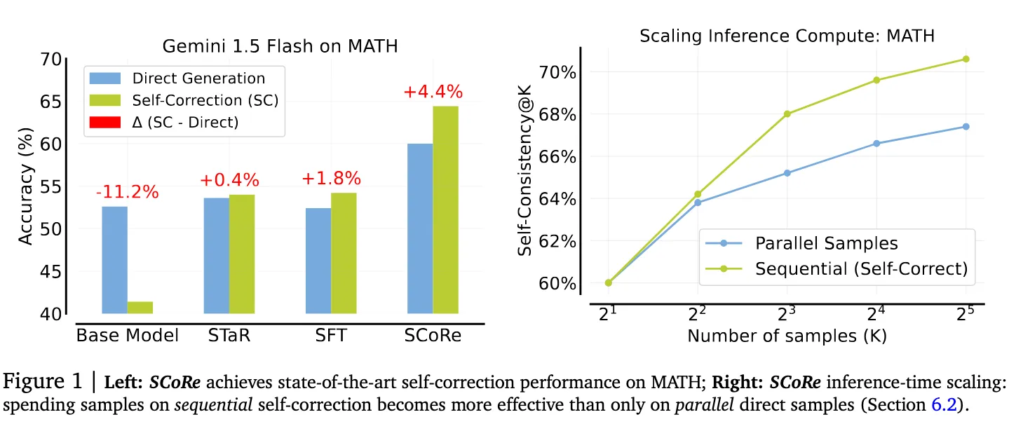
- SCoRE [39]: Reinforcement learning to self-correct.
- Multiagent Debate [40]:Multiple LLMs propose and debate their individual responses and reasoning processes over multiple rounds to arrive at a common final answer.
- Learning to Correct for QA Reasoning with Black-box LLMs [41]: Uses a trained adaptation model to perform a seq2seq mapping imperfect reasonings to the correct or improved reasonings.
- Self-Taught Evaluators [42]: Trains an LLM-as-a-judge using contrasting pairs of synthetically generated model outputs from unlabeled instructions.
For an in-depth survey of the literature on learning to correct, see [43].
Framework: Self-Correction
A simple approach under this self-correction framework is to isolate pairs of chain of thoughts, where one is better than the other, and train a model to improve upon the worse one.
Composed of pairs, where is better than , the model is trained to improve upon .
[38]Iteratively trains a corrector by generating hypotheses and corrections, forming value-improving pairs, and selecting those with high similarity for learning.
- Aim: Find similar CoT pairs where is better
- Train the model to improve upon
Self-taught Evaluators
This notion of creating contrasting pairs as synthetic data has made its way into training model evaluators or so-called LLM-as-a-judge [42].
This paper proposes an iterative self-improvement scheme using synthetic data, where contrasting model outputs from unlabeled instructions are generated. In other words, for each user instruction (example), a preference pair of two model responses (chosen and rejected), is generated via prompting such that the rejected response is likely of lower quality than the chosen response. The approach then trains an LLM-as-a-judge to produce reasoning traces and judgements.
Challenges: Learning Correction
- Collapse: Model may learn to just ignore the negative
- Distribution Shift: Actual mistakes may deviate from examples
Training Language Models to Self-Correct via Reinforcement Learning (SCoRe)
A multi-turn online reinforcement learning approach is proposed to significantly improve and LLM’s self-correction ability using entirely self-generated data.
They found that existing challenges that make it difficult to instill self-correcting behavior in LLMs with variants of supervised fine-tuning SFT alone (like previous works).
SCoRe Training Details
SCoRe Training Details
Empirical Results
When done correctly, this approach beats both training on examples as well as our guess and check approach. It also scales better than simply pairing up examples and learning to correct from them.
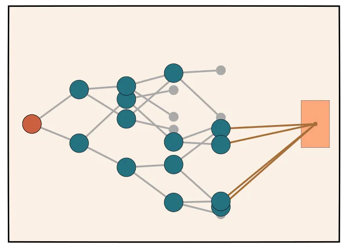
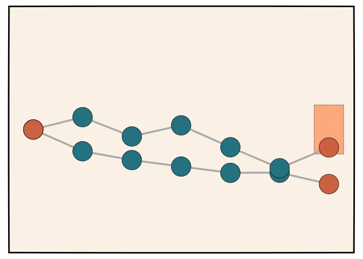
Generalization: Stream of Search [7]
Of course, our final goal is not really individual corrections, but numerous corrections applied repeatedly, all in a single chain as the model explores the space of possible solutions and hones in on the correct one.
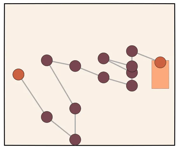
The idea is that you first explore multiple paths using tree search. Then, you convert this stream into a linear sequence by correcting dead-ends back onto paths that lead to the correct answer.
- Find as optimal length CoT with tree search (top graph)
- Find with through backtracking tree search (bottom graph)
- Train on
From Tree to Stream
- Tree search explores multiple paths
- Stream presents a linear sequence
- Allows model to make mistakes in stream

Is this o1?
Considering the pros and cons:
- ✓ Learns to correct and plan
- ✓ Single test-time model
- × Complex training process
- × Limited empirical evidence
Overall, this approach is a bit more complex than simple guess+check and process rewards, but it’s not incompatible and it does seem plausible that this method can be used to induce search-like behavior into a single test time model.
Open o1’s
LLaVA-o1
The recent work LLaVA-o1: Let Vision Language Models Reason Step-by-Step [44] presents an open-source visual language model (VLM) that employs a fixed multistage process involving:
- Summary: A brief outline in which the model summarizes the forthcoming task.
- Caption: A description of the relevant parts of an image (if present), focusing on elements related to the question.
- Logical Reasoning: A detailed analysis in which the model systematically considers the question.
- Conclusion: A concise summary of the answer, providing a final response based on the preceding reasoning.
This structured output approach significantly enhances its ability to systematically tackle complex reasoning problems.
Key Points
The model’s key innovation lies in its staged reasoning framework:
- Independent Processing of Each Stage: By independently processing each reasoning step, the model minimizes common issues such as premature conclusions or logical errors during inference.
- Stage-Level Beam Search: LLaVA-o1 uses a novel stage-level beam search approach at inference time, which generates multiple candidate results at each stage and selects the best one. This provides more robust performance scaling compared to traditional methods like best-of-N or sentence-level beam search.
- Self-Verification: Unlike some existing models that use external verifiers, LLaVA-o1 does not rely on an external or learned verifier during training or inference. Instead, it leverages its structured reasoning stages for self-verification.
- Training Method: LLaVA-o1 was trained using supervised fine-tuning (SFT) on a newly compiled dataset, LLaVA-o1-100k.
- Dataset: The dataset was generated through a multistage reasoning process using GPT-4o, providing structured reasoning annotations from several widely-used visual question-answering (VQA) datasets, including: ShareGPT4V, ChartQA, ScienceQA.
Despite using only 100k training samples, LLaVA-o1 surpasses many larger and even some closed-source models across various multimodal benchmarks, indicating its effectiveness in reasoning-heavy scenarios.
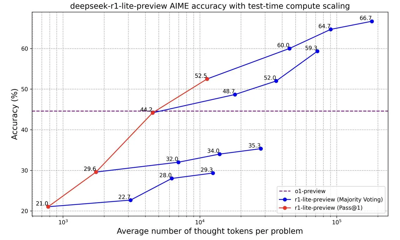
DeepSeek-R1-Lite-Preview [8]
While we don’t have any details on how this model is trained, we are provided with a similar scaling law plot:
Marco-o1 [9]
Overview
🎯 Marco-o1 not only focuses on disciplines with standard answers, such as mathematics, physics, and coding—which are well-suited for reinforcement learning (RL)—but also places greater emphasis on open-ended resolutions. The MarcoPolo Team aims to address the question:
“Can the o1 model effectively generalize to broader domains where clear standards are absent and rewards are challenging to quantify?”
Currently, Marco-o1 Large Language Model (LLM) is powered by Chain-of-Thought (CoT) fine-tuning, Monte Carlo Tree Search (MCTS), reflection mechanisms, and innovative reasoning strategies—optimized for complex real-world problem-solving tasks.
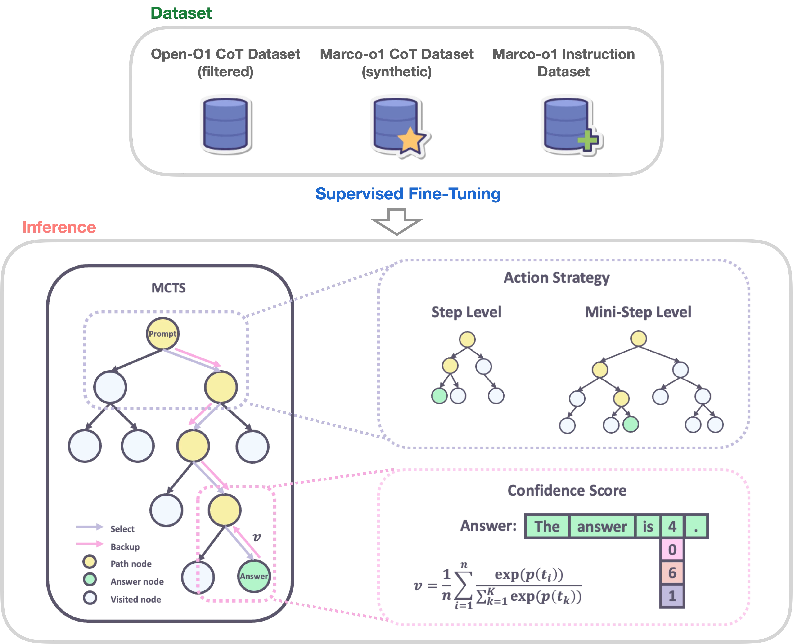
Overview of Marco-o1: A Large Language Model for Open-Ended Problem Solving [9]
Highlights
Currently, Marco-o1 is distinguished by the following highlights:
- 🍀 Fine-Tuning with CoT Data: Marco-o1-CoT undergoes full-parameter fine-tuning on the base model using open-source CoT dataset combined with our self-developed synthetic data.
- 🍀 Solution Space Expansion via MCTS: Integrates MCTS (Marco-o1-MCTS), using the model’s output confidence to guide the search and expand the solution space.
- 🍀 Reasoning Action Strategy: novel reasoning action strategies and a reflection mechanism (Marco-o1-MCTS mini-step), including exploring different action granularities within the MCTS framework and prompting the model to self-reflect, thereby significantly enhancing the model’s ability to solve complex problems.
- 🍀 Application in Translation Tasks: apply Large Reasoning Models (LRM) to Machine Translation task, exploring inference time scaling laws in the multilingual and translation domain.
- [Coming Soon]: Reward models
- [Coming Soon]: Reinforcement learning
Marco Reasoning Datasets
📚 Marco Reasoning Datasets
To enhance the reasoning capabilities of the Marco-o1 model, employed a SFT strategy using a variety of datasets.
-
📊 Open-O1 CoT Dataset (Filtered): Refined Open-O1 project’s CoT Dataset by applying heuristic and quality filtering processes. This enhancement allowed the model to adopt structured reasoning patterns effectively.
-
📊 Marco-o1 CoT Dataset (Synthetic): Generated the Marco-o1 CoT Dataset using MCTS, which helped to formulate complex reasoning pathways, further bolstering the model’s reasoning capabilities.
-
📊 Marco Instruction Dataset: Recognizing the critical role of robust instruction-following capabilities in executing complex tasks, the team incorporated a set of instruction-following data. This integration ensures the model remains competent across a wide range of tasks, maintaining its general effectiveness while significantly boosting its reasoning flair.
| Dataset | #Samples |
|---|---|
| Open-O1 CoT Dataset (Filtered) | 45,125 |
| Marco-o1 CoT Dataset (Synthetic) | 10,000 |
| Marco Instruction Dataset | 5,141 |
| Total | 60,266 |
📥 Marco Reasoning Dataset (Our Partial Dataset)
Solution Space Expansion via MCTS
🌟 Solution Space Expansion via MCTS
The team integrated LLMs with MCTS to enhance the reasoning capabilities of our Marco-o1 model:
- 💎 Nodes as Reasoning States: In the MCTS framework, each node represents a reasoning state of the problem-solving process.
- 💎 Actions as LLM Outputs: The possible actions from a node are the outputs generated by the LLM. These outputs represent potential steps or mini-steps in the reasoning chain.
- 💎 Rollout and Reward Calculation: During the rollout phase, the LLM continues the reasoning process to a terminal state.
- 💎 Guiding MCTS: This reward score is used to evaluate and select promising paths within the MCTS, effectively guiding the search towards more confident and reliable reasoning chains.
Furthermore, the value of each state is obtained by computing a confidence score using the following formulas:
-
Confidence Score ():
For each token generated during the rollout, they calculate its confidence score by applying the softmax function to its log probability and the log probabilities of the top 5 alternative tokens. This is given by:
where:
- is the confidence score for the token in the rollout.
- is the log probability of the token generated by the LLM.
- for to are the log probabilities of the top 5 predicted tokens at the step.
- is the total number of tokens in the rollout sequence.
This equation ensures that the confidence score reflects the relative probability of the chosen token compared to the top alternatives, effectively normalizing the scores between 0 and 1.
-
Reward Score ():
After obtaining the confidence scores for all tokens in the rollout sequence, they compute the average confidence score across all tokens to derive the overall reward score:
where: is the overall reward score for the rollout path.
This average serves as the reward signal that evaluates the quality of the reasoning path taken during the rollout. A higher indicates a more confident and likely accurate reasoning path.
By employing this method, they effectively expand the solution space, allowing the model to explore a vast array of reasoning paths and select the most probable ones based on calculated confidence scores.
Reasoning Action Strategy
🌟 Reasoning Action Strategy
✨ Action Selection
The MarcoPolo team observed that using actions as the granularity for MCTS search is relatively coarse, often causing the model to overlook nuanced reasoning paths crucial for solving complex problems. To address this, they explored different levels of granularity in the MCTS search. Initially, they used steps as the unit of search. To further expand the model’s search space and enhance its problem-solving capabilities, we experimented with dividing these steps into smaller units of 64 or 32 tokens, referred to as “mini-step.” This finer granularity allowed the model to explore reasoning paths in greater detail. While token-level search offers theoretical maximum flexibility and granularity, it is currently impractical due to the significant computational resources required and the challenges associated with designing an effective reward model at this level.
In our experiments, they implemented the following strategies within the MCTS framework:
-
💎 step as Action: They allowed the model to generate complete reasoning steps as actions. Each MCTS node represents an entire thought or action label. This method enables efficient exploration but may miss finer-grained reasoning paths essential for complex problem-solving.
-
💎 mini-step as Action: They used mini-steps of 32 or 64 tokens as actions. This finer granularity expands the solution space and improves the model’s ability to navigate complex reasoning tasks by considering more nuanced steps in the search process. By exploring the solution space at this level, the model is better equipped to find correct answers that might be overlooked with larger action units.
✨ Reflection after Thinking
They introduced a reflection mechanism by adding the phrase “Wait! Maybe I made some mistakes! I need to rethink from scratch.” at the end of each thought process. This prompts the model to self-reflect and reevaluate its reasoning steps. Implementing this reflection has yielded significant improvements, especially on difficult problems that the original model initially solved incorrectly. With the addition of reflection, approximately half of these challenging problems were answered correctly.
From the self-critic perspective, this approach allows the model to act as its own critic, identifying potential errors in its reasoning. By explicitly prompting the model to question its initial conclusions, they encourage it to re-express and refine its thought process. This self-critical mechanism leverages the model’s capacity to detect inconsistencies or mistakes in its own output, leading to more accurate and reliable problem-solving. The reflection step serves as an internal feedback loop, enhancing the model’s ability to self-correct without external intervention.
QwQ: Reflect Deeply on the Boundaries of the Unknown [10]
The Qwen team releases QwQ-32B-Preview as their latest model targeting o1-like capabilities based on the Qwen2.5 series of models. Note: This is the pronunciation of QwQ: /kwju:/ , similar to the word “quill”. In the team’s own words:
it approaches every problem - be it mathematics, code, or knowledge of our world - with genuine wonder and doubt. QwQ embodies that ancient philosophical spirit: it knows that it knows nothing, and that’s precisely what drives its curiosity. Before settling on any answer, it turns inward, questioning its own assumptions, exploring different paths of thought, always seeking deeper truth.
QwQ demonstrates remarkable performance across these benchmarks:
_ 65.2% on GPQA, showcasing its graduate-level scientific reasoning capabilities _ 50.0% on AIME, highlighting its strong mathematical problem-solving skills _ 90.6% on MATH-500, demonstrating exceptional mathematical comprehension across diverse topics _ 50.0% on LiveCodeBench, validating its robust programming abilities in real-world scenarios.
These results underscore QwQ’s significant advancement in analytical and problem-solving capabilities, particularly in technical domains requiring deep reasoning.
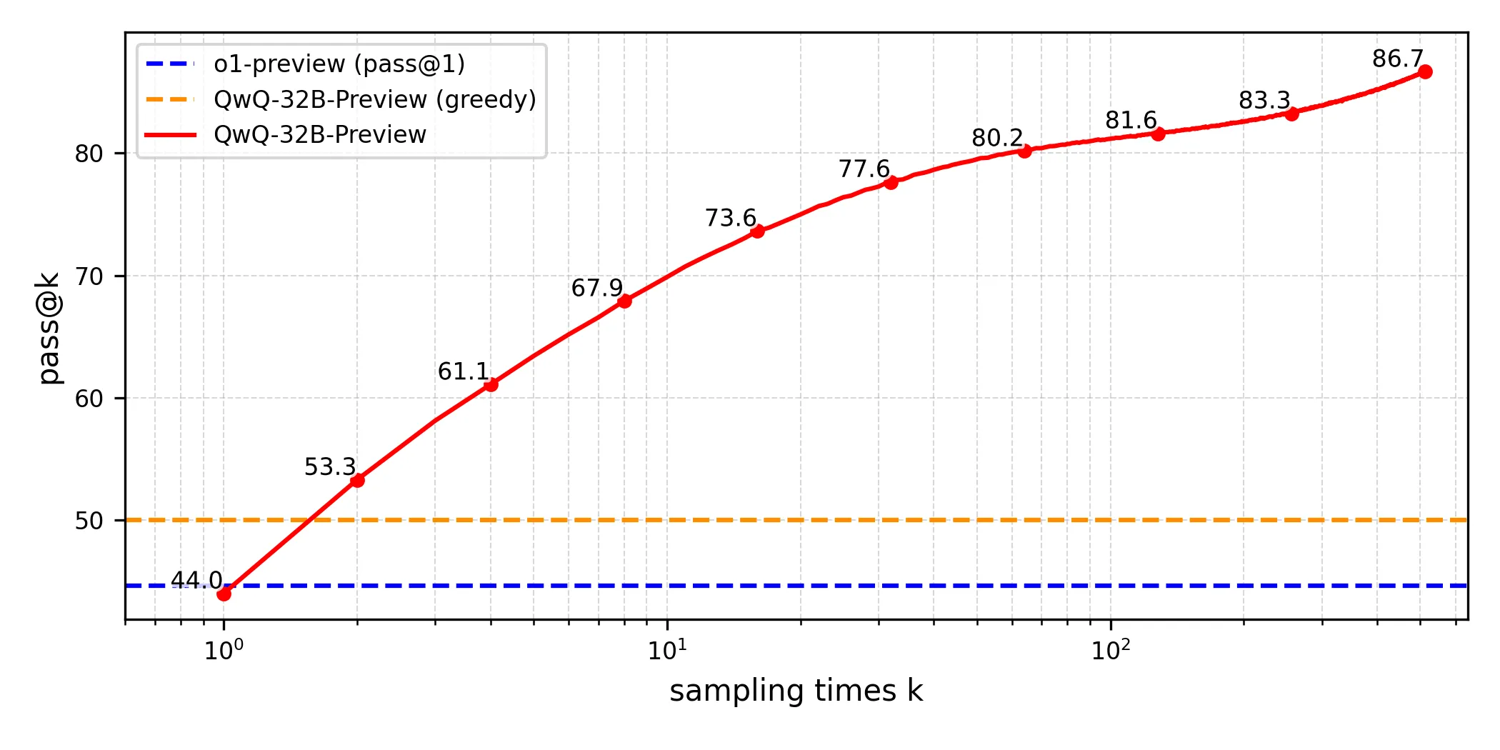
The prototypical test-time scaling curve for QwQ-32B-Preview [10].
What’s next?
Test-time Training
- The surprising effectiveness of test-time training for abstract reasoning [45]
Test-Time Self-Correction with Model Editing
Model editing is exactly as it sounds - the major distinction from say LoRA fine-tuning is that it is a more fine-grained, “surgical” approach to model correction. Specifically, it aims for the adjustment of a model’s behavior for examples within the editing scope while leaving its behavior for out-of-scope examples unaltered.
This technique has been applied to update LLMs’ outdated knowledge and address false associations. However, challenges like limited generalization [46] and unintended side effects persist [47].
In the context of self-correction, model editing appears to be underexplored yet offers great potential for test-time learning, especially if some of the existing challenges are addressed. It enables accurate, fine-grained corrections without full-scale retraining - afterall, humans can update their knowledge or correct mistakes swiftly without having to do a huge amount of relearning! Analyzing the impact of these model edits could yield insights into self-correction. Techniques mitigating model editing’s side effects (Hoelscher-Obermaier et al., 2023) may also enhance self-correction. We anticipate future research to increasingly merge model editing with LLM self-correction, a relatively untouched domain.
References
[1] GitHub - srush/awesome-o1: A bibliography and survey of the papers surrounding o1 — github.com. (n.d.). https://github.com/srush/awesome-o1
[2] Qin, Y., Li, X., Zou, H., Liu, Y., Xia, S., Huang, Z., Ye, Y., Yuan, W., Liu, H., Li, Y., & Liu, P. (2024). O1 Replication Journey: A strategic progress report – part 1.
[3] Uesato, J., Kushman, N., Kumar, R., Song, F., Siegel, N., Wang, L., Creswell, A., Irving, G., & Higgins, I. (2022). Solving math word problems with process- and outcome-based feedback. arXiv [Cs.LG]. http://arxiv.org/abs/2211.14275
[4] Lightman, H., Kosaraju, V., Burda, Y., Edwards, H., Baker, B., Lee, T., Leike, J., Schulman, J., Sutskever, I., & Cobbe, K. (2023). Let’s verify step by step. arXiv [Cs.LG]. http://arxiv.org/abs/2305.20050
[5] Luo, H., Sun, Q., Xu, C., Zhao, P., Lou, J., Tao, C., Geng, X., Lin, Q., Chen, S., & Zhang, D. (2023). WizardMath: Empowering mathematical reasoning for large language models via reinforced Evol-instruct.
[6] Zhang, L., Hosseini, A., Bansal, H., Kazemi, M., Kumar, A., & Agarwal, R. (2024). Generative verifiers: Reward modeling as next-token prediction. arXiv [Cs.LG]. http://arxiv.org/abs/2408.15240
[7] Gandhi, K., Lee, D., Grand, G., Liu, M., Cheng, W., Sharma, A., & Goodman, N. D. (2024). Stream of search (SoS): Learning to search in language. arXiv [Cs.LG]. http://arxiv.org/abs/2404.03683
[8] 🚀 DeepSeek-R1-Lite-Preview is now live: unleashing supercharged reasoning power! (n.d.). https://api-docs.deepseek.com/news/news1120/
[9] Yu, Z., Huifeng, Y., Bo, Z., Hao, W., Tianqi, S., Chenyang, L., Longyue, W., Weihua, L., & Kaifu, Z. (2024). Marco-o1: Towards open reasoning models for open-ended solutions.
[10] Team, Q. (2024). QwQ: Reflect Deeply on the Boundaries of the Unknown. https://qwenlm.github.io/blog/qwq-32b-preview/
[11] - YouTube — youtube.com. (n.d.). https://www.youtube.com/watch?v=jPluSXJpdrA&ab_channel=SequoiaCapital
[12] Brown, T. B., Mann, B., Ryder, N., Subbiah, M., Kaplan, J., Dhariwal, P., Neelakantan, A., Shyam, P., Sastry, G., Askell, A., Agarwal, S., Herbert-Voss, A., Krueger, G., Henighan, T., Child, R., Ramesh, A., Ziegler, D. M., Wu, J., Winter, C., … Amodei, D. (2020). Language Models are Few-Shot Learners.
[13] Kaplan, J., McCandlish, S., Henighan, T., Brown, T. B., Chess, B., Child, R., Gray, S., Radford, A., Wu, J., & Amodei, D. (2020). Scaling laws for neural language models.
[14] Sutton, R. (2019). The Bitter Lesson. In Incomplete Ideas (blog). cs.utexas.edu. https://www.cs.utexas.edu/~eunsol/courses/data/bitter_lesson.pdf
[15] Jones, A. L. (2021). Scaling scaling laws with board games. arXiv [Cs.LG]. http://arxiv.org/abs/2104.03113
[16] Wang, X., Wei, J., Schuurmans, D., Le, Q., Chi, E., Narang, S., Chowdhery, A., & Zhou, D. (2022). Self-Consistency Improves Chain of Thought Reasoning in Language Models. arXiv [Cs.CL]. http://arxiv.org/abs/2203.11171
[17] Nye, M., Andreassen, A. J., Gur-Ari, G., Michalewski, H., Austin, J., Bieber, D., Dohan, D., Lewkowycz, A., Bosma, M., Luan, D., Sutton, C., & Odena, A. (2021). Show your work: Scratchpads for intermediate computation with language models. arXiv [Cs.LG]. http://arxiv.org/abs/2112.00114
[18] Wei, J., Wang, X., Schuurmans, D., Bosma, M., Ichter, B., Xia, F., Chi, E., Le, Q., & Zhou, D. (2022). Chain-of-thought prompting elicits reasoning in large language models. arXiv [Cs.CL], 24824–24837. https://proceedings.neurips.cc/paper_files/paper/2022/file/9d5609613524ecf4f15af0f7b31abca4-Paper-Conference.pdf
[19] Yao, S., Yu, D., Zhao, J., Shafran, I., Griffiths, T. L., Cao, Y., & Narasimhan, K. (2023). Tree of thoughts: Deliberate problem solving with large language models. arXiv [Cs.CL]. http://arxiv.org/abs/2305.10601
[20] Cobbe, K., Kosaraju, V., Bavarian, M., Chen, M., Jun, H., Kaiser, L., Plappert, M., Tworek, J., Hilton, J., Nakano, R., Hesse, C., & Schulman, J. (2021). Training verifiers to solve math word problems. arXiv [Cs.LG]. http://arxiv.org/abs/2110.14168
[21] Welleck, S., Bertsch, A., Finlayson, M., Schoelkopf, H., Xie, A., Neubig, G., Kulikov, I., & Harchaoui, Z. (2024). From decoding to meta-generation: Inference-time algorithms for large language models. arXiv [Cs.CL]. http://arxiv.org/abs/2406.16838
[22] Hendrycks, D., Basart, S., Kadavath, S., Mazeika, M., Arora, A., Guo, E., Burns, C., Puranik, S., He, H., Song, D., & Steinhardt, J. (2021). Measuring coding challenge competence with APPS. arXiv [Cs.SE]. http://arxiv.org/abs/2105.09938
[23] Hendrycks, D., Burns, C., Basart, S., Zou, A., Mazeika, M., Song, D., & Steinhardt, J. (2021). Measuring Massive Multitask Language Understanding. In arXiv [cs.CY]. http://arxiv.org/abs/2009.03300
[24] Anthony, T., Tian, Z., & Barber, D. (2017). Thinking fast and slow with deep learning and tree search. arXiv [Cs.AI]. http://arxiv.org/abs/1705.08439
[25] Yarowsky, D. (1995). Unsupervised word sense disambiguation rivaling supervised methods. Proceedings of the 33rd Annual Meeting on Association for Computational Linguistics -. https://dl.acm.org/doi/10.3115/981658.981684
[26] Zelikman, E., Wu, Y., Mu, J., & Goodman, N. D. (2022). STaR: Bootstrapping reasoning with reasoning. arXiv [Cs.LG]. http://arxiv.org/abs/2203.14465
[27] Gulcehre, C., Paine, T. L., Srinivasan, S., Konyushkova, K., Weerts, L., Sharma, A., Siddhant, A., Ahern, A., Wang, M., Gu, C., Macherey, W., Doucet, A., Firat, O., & de Freitas, N. (2023). Reinforced Self-training (ReST) for language modeling. arXiv [Cs.CL]. https://scholar.google.com/citations?view_op=view_citation&hl=en&citation_for_view=7hwJ2ckAAAAJ:evX43VCCuoAC
[28] Singh, A., Co-Reyes, J. D., Agarwal, R., Anand, A., Patil, P., Garcia, X., Liu, P. J., Harrison, J., Lee, J., Xu, K., Parisi, A., Kumar, A., Alemi, A., Rizkowsky, A., Nova, A., Adlam, B., Bohnet, B., Elsayed, G., Sedghi, H., … Fiedel, N. (2023). Beyond human data: Scaling self-training for problem-solving with language models. arXiv [Cs.LG]. http://arxiv.org/abs/2312.06585
[29] Nakano, R., Hilton, J., Balaji, S., Wu, J., Ouyang, L., Kim, C., Hesse, C., Jain, S., Kosaraju, V., Saunders, W., Jiang, X., Cobbe, K., Eloundou, T., Krueger, G., Button, K., Knight, M., Chess, B., & Schulman, J. (2021). WebGPT: Browser-assisted question-answering with human feedback. arXiv [Cs.CL]. http://arxiv.org/abs/2112.09332
[30] Hosseini, A., Yuan, X., Malkin, N., Courville, A., Sordoni, A., & Agarwal, R. (2024). V-STaR: Training Verifiers for Self-Taught Reasoners.
[31] Wang, P., Li, L., Shao, Z., Xu, R. X., Dai, D., Li, Y., Chen, D., Wu, Y., & Sui, Z. (2023). Math-Shepherd: Verify and reinforce LLMs step-by-step without human annotations. arXiv [Cs.AI]. http://arxiv.org/abs/2312.08935
[32] Ma, Q., Zhou, H., Liu, T., Yuan, J., Liu, P., You, Y., & Yang, H. (2023). Let’s reward step by step: Step-Level reward model as the Navigators for Reasoning.
[33] Su, D., Sukhbaatar, S., Rabbat, M., Tian, Y., & Zheng, Q. (2024). Dualformer: Controllable fast and slow thinking by learning with randomized reasoning traces. arXiv [Cs.AI]. http://arxiv.org/abs/2410.09918
[34] Feng, X., Wan, Z., Wen, M., McAleer, S. M., Wen, Y., Zhang, W., & Wang, J. (2023). Alphazero-like tree-search can guide large language model decoding and training. arXiv [Cs.LG]. http://arxiv.org/abs/2309.17179
[35] Xie, Y., Goyal, A., Zheng, W., Kan, M.-Y., Lillicrap, T. P., Kawaguchi, K., & Shieh, M. (2024). Monte Carlo Tree Search boosts reasoning via iterative preference learning. arXiv [Cs.AI]. http://arxiv.org/abs/2405.00451
[36] Putta, P., Mills, E., Garg, N., Motwani, S., Finn, C., Garg, D., & Rafailov, R. (2024). Agent Q: Advanced reasoning and learning for autonomous AI agents. arXiv [Cs.AI]. http://arxiv.org/abs/2408.07199
[37] Setlur, A., Nagpal, C., Fisch, A., Geng, X., Eisenstein, J., Agarwal, R., Agarwal, A., Berant, J., & Kumar, A. (2024). Rewarding progress: Scaling automated process verifiers for LLM reasoning. arXiv [Cs.LG]. http://arxiv.org/abs/2410.08146
[38] Welleck, S., Lu, X., West, P., Brahman, F., Shen, T., Khashabi, D., & Choi, Y. (2022). Generating sequences by learning to Self-correct. arXiv [Cs.CL]. http://arxiv.org/abs/2211.00053
[39] Kumar, A., Zhuang, V., Agarwal, R., Su, Y., Co-Reyes, J. D., Singh, A., Baumli, K., Iqbal, S., Bishop, C., Roelofs, R., Zhang, L. M., McKinney, K., Shrivastava, D., Paduraru, C., Tucker, G., Precup, D., Behbahani, F., & Faust, A. (2024). Training language models to self-correct via reinforcement learning. arXiv [Cs.LG]. http://arxiv.org/abs/2409.12917
[40] Du, Y., Li, S., Torralba, A., Tenenbaum, J. B., & Mordatch, I. (2023). Improving factuality and reasoning in language models through multiagent debate.
[41] Kim, J., Kim, D., & Yang, Y. (2024). Learning to correct for QA reasoning with black-box LLMs.
[42] Wang, T., Kulikov, I., Golovneva, O., Yu, P., Yuan, W., Dwivedi-Yu, J., Pang, R. Y., Fazel-Zarandi, M., Weston, J., & Li, X. (2024). Self-Taught Evaluators.
[43] Pan, L., Saxon, M., Xu, W., Nathani, D., Wang, X., & Wang, W. Y. (2024). Automatically Correcting Large Language Models: Surveying the Landscape of Diverse Automated Correction Strategies. Transactions of the Association for Computational Linguistics, 12, 484–506. https://doi.org/10.1162/tacl_a_00660
[44] Xu, G., Jin, P., Hao, L., Song, Y., Sun, L., & Yuan, L. (2024). LLaVA-o1: Let Vision Language Models reason step-by-step.
[45] Akyürek, E., Damani, M., Qiu, L., Guo, H., Kim, Y., & Andreas, J. (2024). The surprising effectiveness of test-time training for abstract reasoning.
[46] Yao, Y., Wang, P., Tian, B., Cheng, S., Li, Z., Deng, S., Chen, H., & Zhang, N. (2023). Editing large language models: Problems, methods, and opportunities.
[47] Hoelscher-Obermaier, J., Persson, J., Kran, E., Konstas, I., & Barez, F. (2023). Detecting edit failures in large language models: An improved specificity benchmark.