Neural Scaling Laws
For better or worse, it certainly feels like OpenAI has been in the news a lot lately, almost daily it seems. The intense spotlight on the company isn’t without reason, however. Researchers there have a long track-record of pushing the boundaries of what’s possible in AI, and their work has largely shaped the entire agenda of the field. Historically, their graphs really have moved the needle (excuse my corporate parlance).
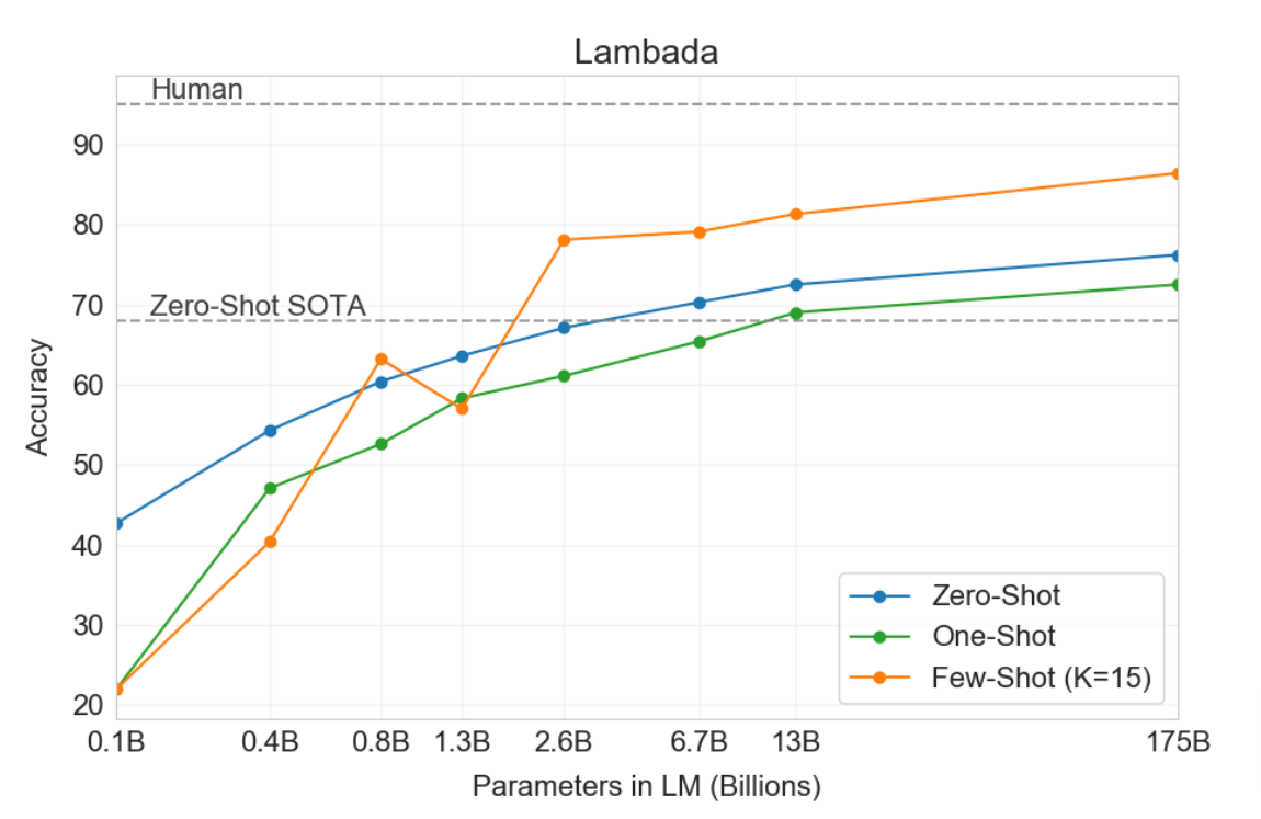
This graph on the left is from the GPT-3 paper [1], and it’s one of several that demonstrate that as the number of parameters in a language model increases, so does its zero-shot performance on downstream tasks. This graph, and many others like it, has occupied the interest of the language modeling community for the last five years. It really changed the way we think about many different problems and how we build, design, scale, and invest in models. Spoiler alert:… Bigger has been better…sighs In fact, right now, it’s safe to say that there are nuclear power plants being built just to support this graph.
TL; DR
-
Early scaling laws (Kaplan et al., 2020) established power-law relationships between model size, data, and performance.
-
The Chinchilla paradigm shift (2022) introduced the 20:1 token-to-parameter ratio for optimal training.
-
Post-Chinchilla developments saw “overtraining” beyond the 20:1 ratio, yielding performance gains.
-
Recent models like Llama-3 pushed token-to-parameter ratios to 200:1, challenging previous assumptions.
-
Inference scaling (OpenAI’s o1 model, 2024) emerged as a new direction, focusing on optimizing inference-time compute for improved reasoning.
What are Scaling Laws?
A language model is characterized by about 4 main elements:
- - The number of parameters in the model, which represents the ability of the model to learn from the data. A model with more parameters has more flexibility to capture complex patterns in the data.
- : The size of the training dataset measured in number of tokens (a small piece of text, ranging from a few words to a single character).
- : The compute budget used to train it (measured in FLOPs or floating point operations per second).
The network architecture (we assume that all current powerful LLMs are based on the Transformer architecture). It is now well known that increasing the number of parameters leads to better performance in a wide range of linguistic tasks. Some models like PaLM exceed 540 billion parameters.
The question is therefore: Given a fixed increase in the compute budget, in what proportion should we increase the number of parameters and the size of the training dataset to achieve the optimal loss ?
Interlude: Estimating Transformer Properties
In order to really appreciate neural scaling laws and what they tell us, it’s important to understand how we can estimate the properties of a Transformer model. Here are some of the key properties we can estimate:
- FLOPs
- number of parameters
- peak memory footprint
- checkpoint size
I recommend reading Estimating Transformer Model Properties: A Deep Dive for a more in-depth discussion on how to estimate these properties.
Early Scaling Laws (2020 and before)
OpenAI’s 2020 work on scaling laws [2] jump started investigations into the relationship between model size, data, and performance.
The paper established power-law relationships between these three factors, showing that as the number of parameters in a model increases, so does its performance on a range of tasks. The work also emphasized the importance of increasing the models parameters (3x more important) than expanding the training set size.This work laid the foundation for the subsequent explosion in model sizes and the development of ever-larger language models.
Fitting power laws to the data
Let’s start with one of the key equations from their paper:
- Number of parameters : For models with a limited number of parameters, trained to convergence on a sufficiently large dataset:
where is the number of non-embedding parameters.
- Training data size : For large models trained on a limited dataset with early stopping:
where is the number of tokens in the training set.
- Compute budget : For sufficiently sized datasets and optimally-sized models, the loss given a limited amount of compute scales as:
Critical batch size: Determines the speed/efficiency tradeoff for data parallelism also roughly obeys a power law in :
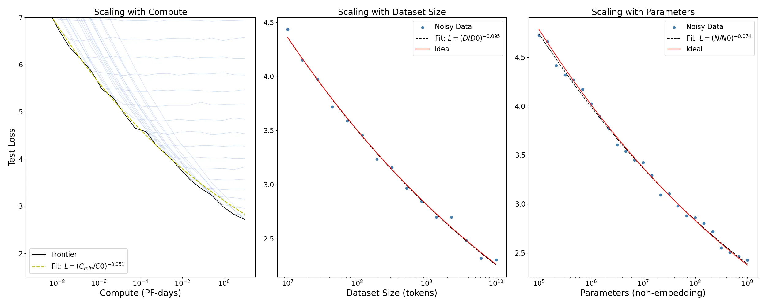
Scaling Laws Figure 1 (reproduced)
Scaling Laws Figure 1 from OpenAI’s 2020 paper
Code for reproducing the scaling laws plots
import matplotlib.pyplot as plt
import numpy as np
from scipy.optimize import curve_fit

#########################
# Synthetic Data Generation
#########################

# Define scaling parameters from the paper-like scenario
C0, D0, N0 = (2.3e8, 5.4e13, 8.8e13)
# reference points (these are from the caption but not exact)
alpha_C, alpha_B, alpha_N = 0.050, 0.095, 0.076  # exponents from the figure notes

# Generate ranges for compute, dataset size, and parameters
C_values = np.logspace(-9, 1, 20)  # from 10^-9 to 10^1 PF-days
D_values = np.logspace(7, 10, 15)  # from 10^7 to 10^10 tokens
N_values = np.logspace(5, 9, 25)  # from 10^5 to 10^9 parameters

# Ideal power-law relationships:
L0 = 1.0  # We'll pick a baseline scale.
L_compute_ideal = L0 * (C_values / C0) ** (-alpha_C)
L_dataset_ideal = L0 * (D_values / D0) ** (-alpha_B)
L_params_ideal = L0 * (N_values / N0) ** (-alpha_N)

# Add some noise to simulate experimental data
noise_scale = 0.05
L_compute_noisy = L_compute_ideal + np.random.normal(
    0, noise_scale, size=len(L_compute_ideal)
)
L_dataset_noisy = L_dataset_ideal + np.random.normal(
    0, noise_scale, size=len(L_dataset_ideal)
)
L_params_noisy = L_params_ideal + np.random.normal(
    0, noise_scale, size=len(L_params_ideal)
)

# Compute training loss curves for multiple runs
# Loss curves should enter plateau at different regions following the scaling laws
curves = []
C_values = np.logspace(-9, 1, 20)  # from 10^-9 to 10^1 PF-days
for i, plateau in enumerate(L_compute_ideal):
    # Slightly vary alpha_C and L0 per run for realism
    alpha_run = alpha_C * (i / 100 + 1 + np.random.normal(0, 0.01))  # ~10% variation
    L0_run = L0 * (1 + np.random.normal(0, 0.001))  # ~5% variation

    # Ideal power-law part
    L_ideal = L0_run * ((C_values) / C0) ** (-alpha_run)

    # Apply a plateau at L_min
    L_run = np.maximum(L_ideal, plateau)

    # Add some random noise
    noise = np.random.normal(0, 0.02, size=len(L_run))
    L_run_noisy = L_run + noise

    curves.append(L_run_noisy)

#########################
# Fitting Power-Laws
#########################


def power_law(x, A, p, x_ref=C0):
    """Power-law fitting function.

    We'll assume the form
        L = A * (x / x_ref)^(-p)
    where A and p are fit parameters (we can hold x_ref fixed)

    """
    return A * (x / x_ref) ** (-p)


fit_region_mask = (C_values < 1e-3) & (C_values > 1e-7)
L_frontier = np.min(np.stack(curves, axis=0), axis=0)

# Fit for compute
popt_compute, pcov_compute = curve_fit(
    lambda x, A, p: power_law(x, A, p, C0), C_values, L_compute_noisy, p0=[L0, alpha_C]
)
A_c, p_c = popt_compute

# Fit for dataset size
popt_dataset, pcov_dataset = curve_fit(
    lambda x, A, p: power_law(x, A, p, D0), D_values, L_dataset_noisy, p0=[L0, alpha_B]
)
A_d, p_d = popt_dataset

# Fit for parameters
popt_params, pcov_params = curve_fit(
    lambda x, A, p: power_law(x, A, p, N0), N_values, L_params_noisy, p0=[L0, alpha_N]
)
A_n, p_n = popt_params

#########################
# Plotting the results
#########################

fig, axs = plt.subplots(1, 3, figsize=(25, 10))

# Plot Compute scaling
# Plot all runs in blue
for run_loss in curves:
    axs[0].plot(C_values, run_loss, color="cornflowerblue", alpha=0.3, linewidth=1)
# Plot the frontier line in black
axs[0].plot(C_values, L_frontier, "k-", label="Frontier")

# Plot the fitted region and curve
C_fine = np.logspace(-9, 1, 200)
L_fitted_curve = power_law(C_fine, A_n, p_c, C0)
axs[0].plot(
    C_fine,
    L_fitted_curve,
    "y--",
    linewidth=2,
    label="Fit: $L = (C_{min}/C0)^{-" f"{p_c:.3f}" "}$",
)

# Set scales and labels
axs[0].set_xscale("log")
axs[0].set_xlabel("Compute (PF-days)")
axs[0].set_ylabel("Test Loss")
axs[0].set_title("Scaling with Compute")
axs[0].set_ylim(1.5, 7)  # limit y-axis to show the plateau
axs[0].legend()

# Plot Dataset scaling
axs[1].scatter(D_values, L_dataset_noisy, label="Noisy Data", color="steelblue")
axs[1].plot(
    D_values,
    power_law(D_values, A_d, p_d, D0),
    "k--",
    label="Fit: $L = (D/D0)^{-" f"{p_d:.3f}" "}$",
)
axs[1].plot(D_values, L_dataset_ideal, "r-", label="Ideal")
axs[1].set_xscale("log")
axs[1].set_xlabel("Dataset Size (tokens)")
axs[1].legend()
axs[1].set_title("Scaling with Dataset Size")

# Plot Parameters scaling
axs[2].scatter(N_values, L_params_noisy, label="Noisy Data", color="steelblue")
axs[2].plot(
    N_values,
    power_law(N_values, A_n, p_n, N0),
    "k--",
    label="Fit: $L = (N/N0)^{-" f"{p_n:.3f}" "}$",
)
axs[2].plot(N_values, L_params_ideal, "r-", label="Ideal")
axs[2].set_xscale("log")
axs[2].set_xlabel("Parameters (non-embedding)")
axs[2].legend()
axs[2].set_title("Scaling with Parameters")


plt.tight_layout()
plt.show()
The Chinchilla Paradigm Shift (2022)
In March 2020, DeepMind published a paper “Training Compute Optimal Large Language models”[3], which introduced what became known as the Chinchilla Scaling law.
The Chinchilla paper asked:
If you have a fixed training compute budget, how should you balance model size and training duration to produce the highest quality model?
From training over 400 LLMs ranging from 70M to 16B parameters on 5-500B tokens, the authors found that:
For compute-optimal training, the model size and the number of tokens should scale equally: doubling the model size should be accompanied by doubling the number of training tokens.
They also introduced the 20:1 token-to-parameter ratio as the optimal balance between model size and training data. This ratio was found to be the most efficient in terms of training time and model quality. In other words, each parameter in the model should be trained on 20 tokens.
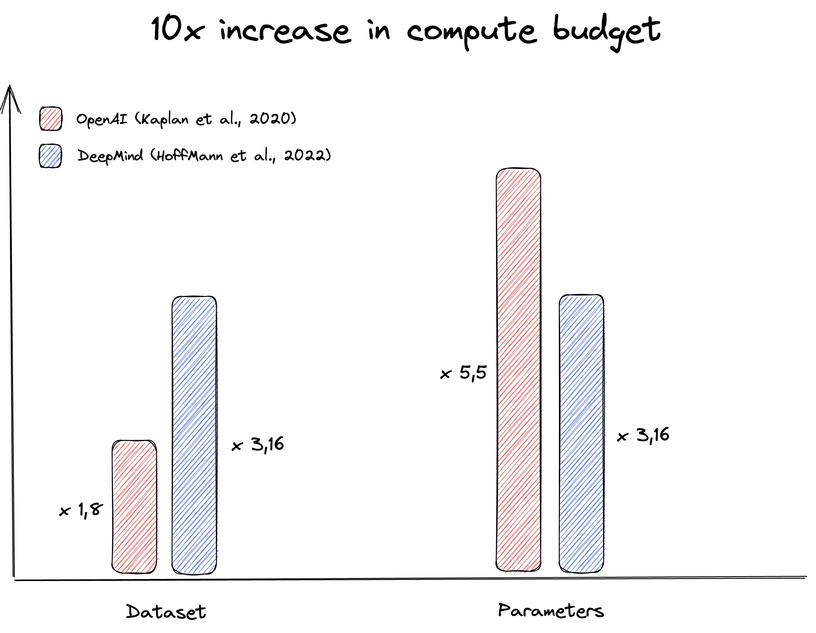
OpenAI Scaling Law vs. Chinchilla Scalling Law source
Chinchilla Scaling in more detail
In the Chinchilla paper, the authors propose 3 approaches to answer the question: “Given a fixed FLOPs budget, how should one trade-off model size and the number of training tokens?”
- Fix model sizes and vary number of training tokens: Directly estimate the minimum loss achieved for a given number of training flops.
- IsoFLOP profiles/curves: Vary the model size for a fixed number (9) of different training FLOP counts and consider the final training loss for each point.
- Fitting a parametric loss function: Following classical risk decomposition, the authors fit a parametric loss function to the data:
Approach 3: Fitting a parametric loss function
Let’s continue unpacking their third approach, which fits a function to approximate the final loss gives the model size and the data size. Here is the final fit:
The parametric function was fitg by minimizing the Huber loss using the L-BFGS-B algorithm:
which produced the following fit:
where is the estimated “entropy of natural language” (the limit of an infinite model on infinite data).
def L(N, D):
    """
    Approximates loss given
    - N parameters and
    - D dataset size (in tokens),
    per Chinchilla paper.
    """
    E = 1.69 # entropy of natural language,
             # limit of inf model on inf data
    A = 406.4
    B = 410.7
    alpha = 0.34
    beta = 0.28
    return A / (N ** alpha) + B / (D ** beta) + E
Given this fit, let’s visualize the loss function for a range of model sizes and dataset sizes:
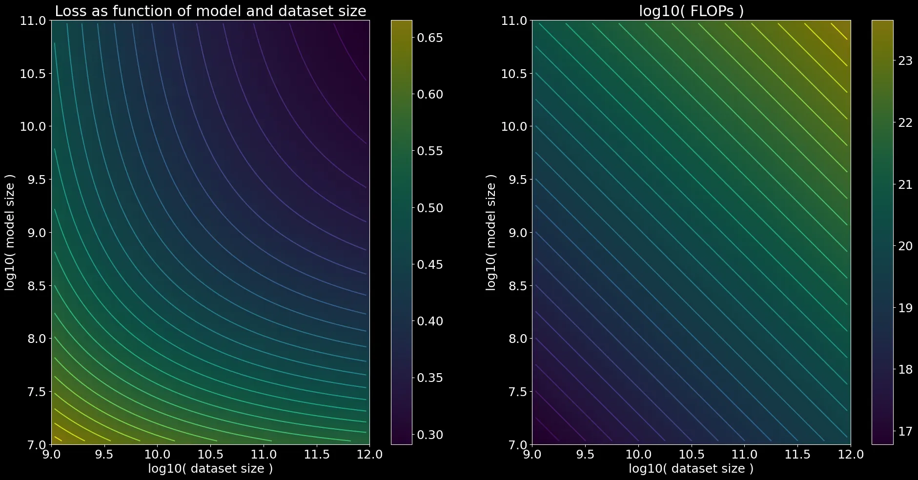
Plotting Code
import matplotlib.pyplot as plt
import numpy as np


def L(N, D):
    """
    Approximates loss given N parameters and D dataset size (in tokens),
    per Chinchilla paper.
    """
    E = 1.69  # entropy of natural language, limit of infinite model on infinite data
    A = 406.4
    B = 410.7
    alpha = 0.34
    beta = 0.28
    return A / (N**alpha) + B / (D**beta) + E


ns = 10 ** np.arange(7, 11, step=2**-4)  # model sizes from 10M to 100B
ds = 10 ** np.arange(9, 12, step=2**-4)  # dataset sizes from 1B to 1T

fig, axs = plt.subplots(1, 2, figsize=(20, 10))

# Create 2D contour plot of loss as function of model size and dataset size
loss2d = np.log10(np.array([[L(n, d) for d in ds] for n in ns]))
im = axs[0].imshow(loss2d, extent=[9, 12, 7, 11], origin="lower", alpha=0.5)
axs[0].contour(loss2d, levels=30, extent=[9, 12, 7, 11], origin="lower")
axs[0].set_xlabel("log10( dataset size )")
axs[0].set_ylabel("log10( model size )")
axs[0].set_title("Loss as function of model and dataset size")
fig.colorbar(im, ax=axs[0])

# Plot the compute for each point: FLOPs = 6 * N * D
compute2d = np.log10([[6 * n * d for d in ds] for n in ns])
im = axs[1].imshow(compute2d, extent=[9, 12, 7, 11], origin="lower", alpha=0.5)
axs[1].contour(compute2d, levels=30, extent=[9, 12, 7, 11], origin="lower")
axs[1].set_xlabel("log10( dataset size )")
axs[1].set_ylabel("log10( model size )")
axs[1].set_title("log10( FLOPs )")
fig.colorbar(im, ax=axs[1])
plt.tight_layout()
plt.savefig("loss2d.png")
Ok so given any we can estimate both:
- the loss
- the total flops.
Now given a specific budget of flops , we want to find:
In other words, how big of a model should we train and for how many tokens?
Iso-Curves Plotting Code
Cs = [
    6e18,
    1e19,
    3e19,
    6e19,
    1e20,
    3e20,
    6e20,
    1e21,
    3e21,
]
# Sweep over model sizes for 10M to 100B
ns = 10 ** np.arange(7, 11, step=2**-4)
plt.figure()
for c in Cs:
	# Using C = 6 * N * D, solve for D = C / (6 * N)
	ds = c / (6 * ns)

	losses = L(ns, ds)
	# find best model size
	best_idx = np.argmin(losses)
	print(f"Best model size: {ns[best_idx]:.2e}, loss: {losses[best_idx]:.2f}")
	print(f"Best dataset size: {ds[best_idx]:.2e}")
	plt.semilogx(ns, losses, label=f"C={c:.2e}")
	# plot a vertical bar at the best model size
	# plt.axvline(ns[best_idx], color="red")

ticks = [1e8, 3e8, 3e9, 6e9, 3e10]
labels = ['100M', '300M', '3B', '6B', '30B']

plt.xticks(ticks)
plt.gca().set_xticklabels(labels)
plt.ylim(2, 3.5)
plt.xlabel("model size")
plt.ylabel("loss")
plt.legend()
plt.title("Iso-loss curves for different compute budgets")
plt.savefig("isocurves.png")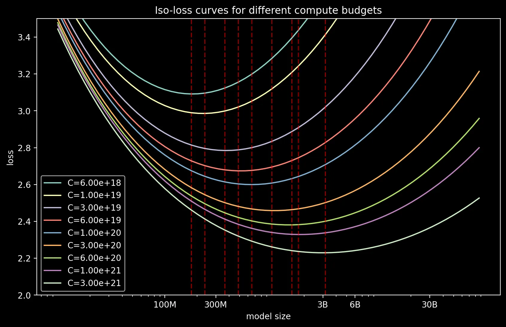
In the plot above, basically the models on the left of best are too small and trained for too long. The models on the right of best are way too large and trained for too little. The model at the red line is just right.
Approach 2
Approach 2 is a fairly direct measurement of what we are after: fix a flop budget and run a number of model/dataset sizes, measure the loss, fit a parabola, and get the minimum.
Then, given a new compute budget, you can interpolate to find the compute-optimal number of tokens for any given model size.
raw = [ # parameters, tokens
    [400e6, 7.7e9],
    [1e9, 20.0e9],
    [10e9, 219.5e9],
    [67e9, 1.7e12],
    [175e9, 4.3e12],
    [280e9, 7.1e12],
    [520e9, 13.4e12],
    [1e12, 26.5e12],
    [10e12, 292.0e12]]
x = np.array([np.log10(r[0]) for r in raw])
y = np.array([np.log10(r[1]) for r in raw])
A = np.vstack([x, np.ones(len(x))]).T
m, c = np.linalg.lstsq(A, y, rcond=None)[0]
print(f"y = {m:.2f}x + {c:.2f}")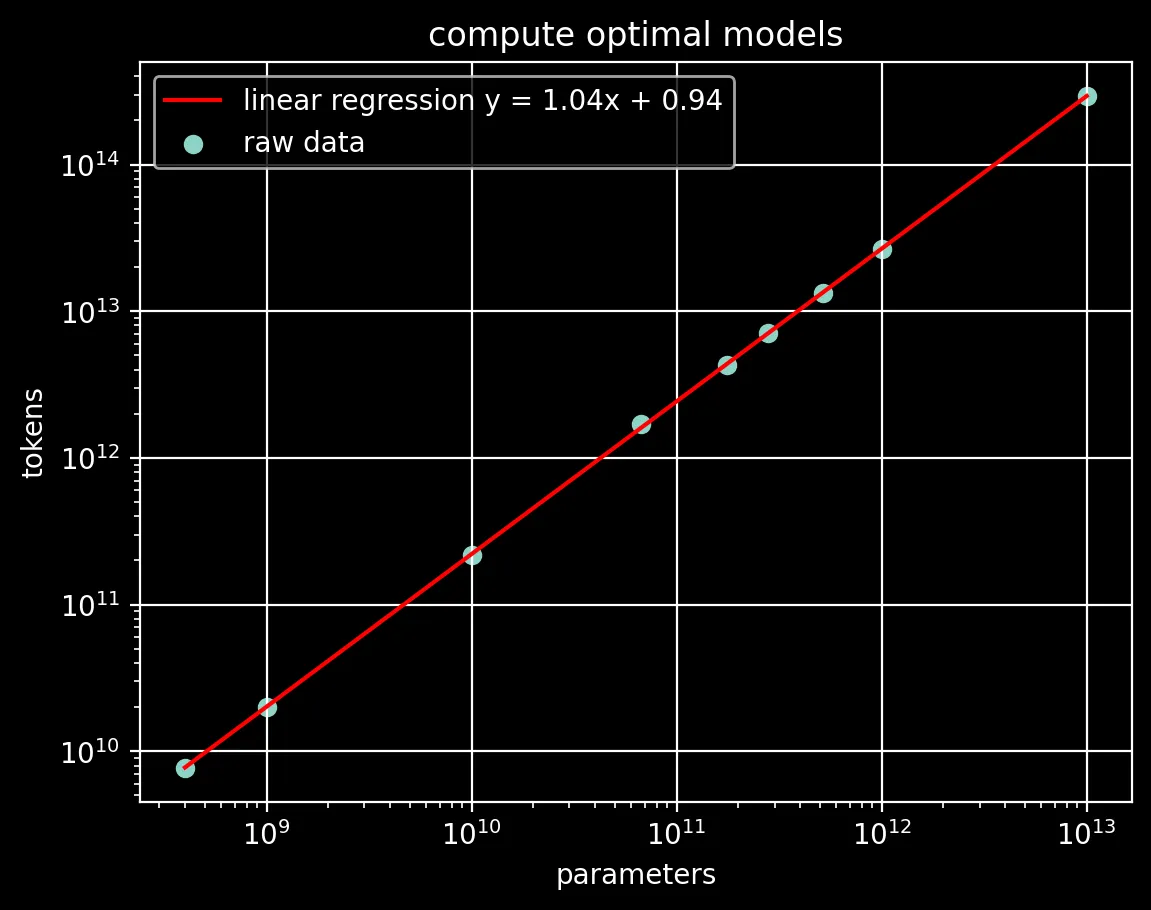
Plotting Code
plt.figure()
# plot the line
plt.plot(
    [q[0] for q in raw],
    [10 ** (m * np.log10(q[0]) + c) for q in raw],
    label=f"linear regression y = {m:.2f}x + {c:.2f}",
    color="r",
)
# plot the raw data
plt.scatter([q[0] for q in raw], [q[1] for q in raw], label="raw data")
plt.xscale("log")
plt.yscale("log")
plt.xlabel("parameters")
plt.ylabel("tokens")
plt.legend()
plt.title("compute optimal models")
plt.grid()
”Overtraining” - Post-Chinchilla Developments (2022-2023)
The Chinchilla paradigm shift was a major milestone in the evolution of scaling laws, but it wasn’t the end of the story. Organizations and researchers continue to probe the subject, challenging assumptions. Meta’s Llama family of models, for example, pushed the token-to-parameter ratio to 200:1. This was a significant departure from the 20:1 ratio established by Chinchilla, and it yielded performance gains.
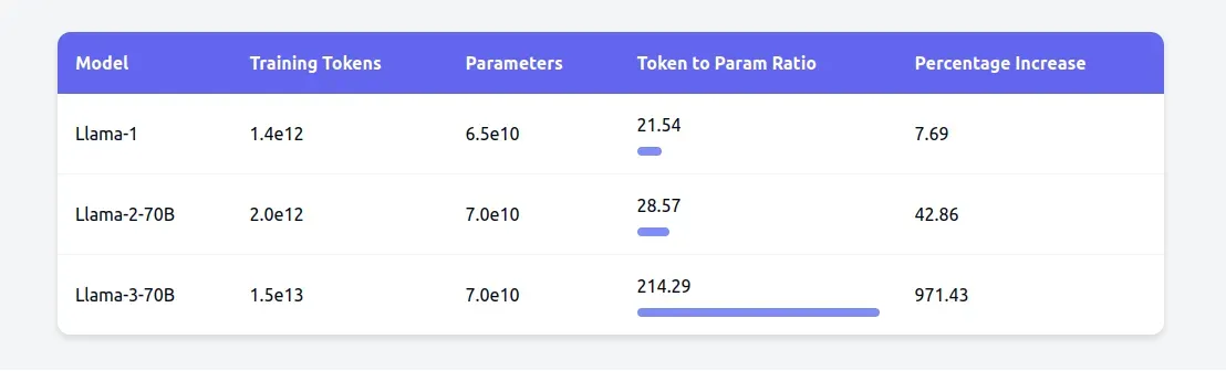
While Llama-1 (65B) adhered closely to the Chinchilla ratio with about 20 tokens per parameter, Llama-2-70B increased this to nearly 30 tokens per parameter. The Llama-3-70B took this further, training on over 200 tokens per parameter, or 15 trillion tokens total. The 8B and 70B parameter models improved log-linearly after training on up to 15T tokens.
There are likely several reasons for this shift towards overtraining:
- Research like the herd of llama models have shown that there is still “meat on the bone” in terms of performance gains from training models for longer.
- There’s a growing demand for more powerful yet smaller models (1-8B) that can be deployed in resource-constrained environments.
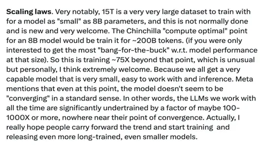
Karpathy’s tweet on overtraining source
Prominent figures in the field, like Andrej Karpathy, have also weighed in, suggesting that today’s models may still be “significantly undertrained.”
The 2024 paper “Beyond Chinchilla-Optimal: Accounting for Inference in Language Model Scaling Laws” [4] further challenge Chinchilla-optimal scaling laws claiming that they neglect the downstream cost of inference. After all, inference compute for widely popular and heavily used models will largely outpace training compute as models are deployed in the real world. This work analyzes both compute budgets and real-world costs, finding that models with reasonably high inference-demand should train models smaller and longer than the Chinchilla-optimal ratio. This insight is likely to become increasingly important in the context of evolving research trends, as we’ll see in the next section.
The Rise of Inference Scaling (2023-2024)
Large companies and research organizations have continued to push the boundaries of pretraining scaling laws, so much so that there are non-ironic discussions about building nuclear power plants to support the compute requirements of these models.
In this context, it is easier to understand why one might turn to other methods for increasing the performance of models that don’t simply rely on increasing the number of parameters. Hence, the shift towards optimizing what you might have heard as “inference-time compute” - which is essentially asking how you can spend more computer at test-time to improve responses as opposed to just training-time.
The o1 Era
In 2024, OpenAI introduced the o1 model, which marked a significant departure from the traditional scaling laws. The o1 model was designed with a focus on optimizing inference-time compute for improved reasoning capabilities. This new direction in scaling laws has opened up exciting possibilities for future research and development in the field of AI.
For an in-depth overview at this line of work, please see another post o1-and-reasoning.
Future Directions
- Optimal token-to-parameter ratios:
- Data quality and efficiency
- Inference-time scaling
References
[1] Brown, T. B., Mann, B., Ryder, N., Subbiah, M., Kaplan, J., Dhariwal, P., Neelakantan, A., Shyam, P., Sastry, G., Askell, A., Agarwal, S., Herbert-Voss, A., Krueger, G., Henighan, T., Child, R., Ramesh, A., Ziegler, D. M., Wu, J., Winter, C., … Amodei, D. (2020). Language Models are Few-Shot Learners.
[2] Kaplan, J., McCandlish, S., Henighan, T., Brown, T. B., Chess, B., Child, R., Gray, S., Radford, A., Wu, J., & Amodei, D. (2020). Scaling laws for neural language models.
[3] Hoffmann, J., Borgeaud, S., Mensch, A., Buchatskaya, E., Cai, T., Rutherford, E., de Las Casas, D., Hendricks, L. A., Welbl, J., Clark, A., Hennigan, T., Noland, E., Millican, K., van den Driessche, G., Damoc, B., Guy, A., Osindero, S., Simonyan, K., Elsen, E., … Sifre, L. (2022). Training Compute-Optimal Large Language Models. arXiv [Cs.CL]. http://arxiv.org/abs/2203.15556
[4] Sardana, N., Portes, J., Doubov, S., & Frankle, J. (2023). Beyond Chinchilla-optimal: Accounting for inference in language model scaling laws.